Space limitations and high power supply requirements ultimately lead to innovative cooling designs for a wide range of PCBs. The arrangement of the power supply, heatsink dimensions, and the design of the outer housing become more important. Thermal simulations within the PCB design process help to overcome overheating problems in later production stages. 

Different materials, the combination of heat conduction, convective, and radiative heat transfer within solids and air result in fairly complex thermal simulations. Setting up material properties, boundary conditions, solver settings, and coupling regions often takes a considerable amount of time.

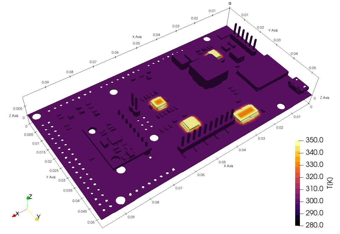
As an example, a typical PCB with its components is presented.

Simulación térmica 

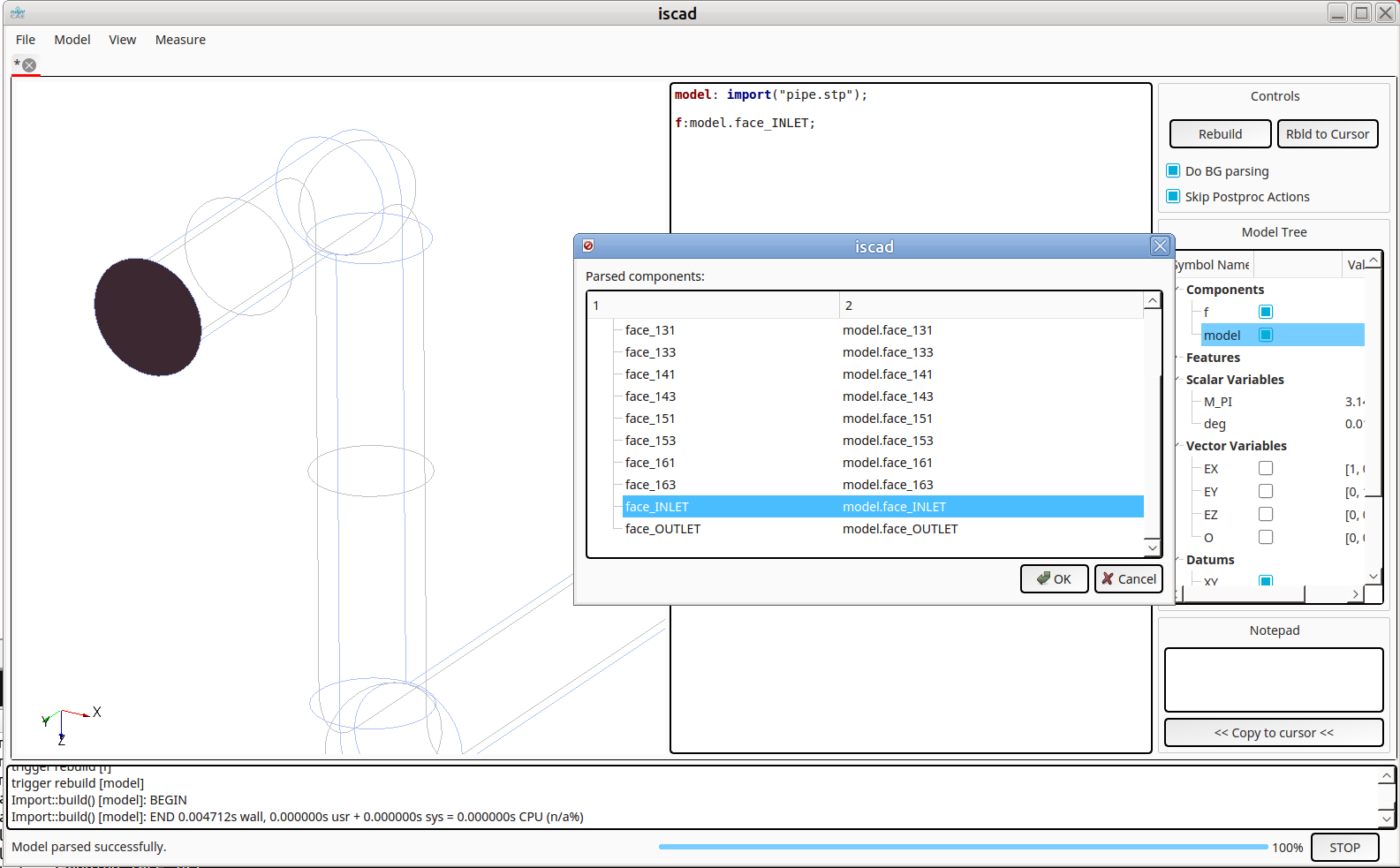
Silentdynamics has managed to bundle the simulation setup using OpenFOAM thermal solverschtMultiRegionFoam,  chtMultiRegionSimpleFoamwithin its framework InsightCAE for fast preprocessing.

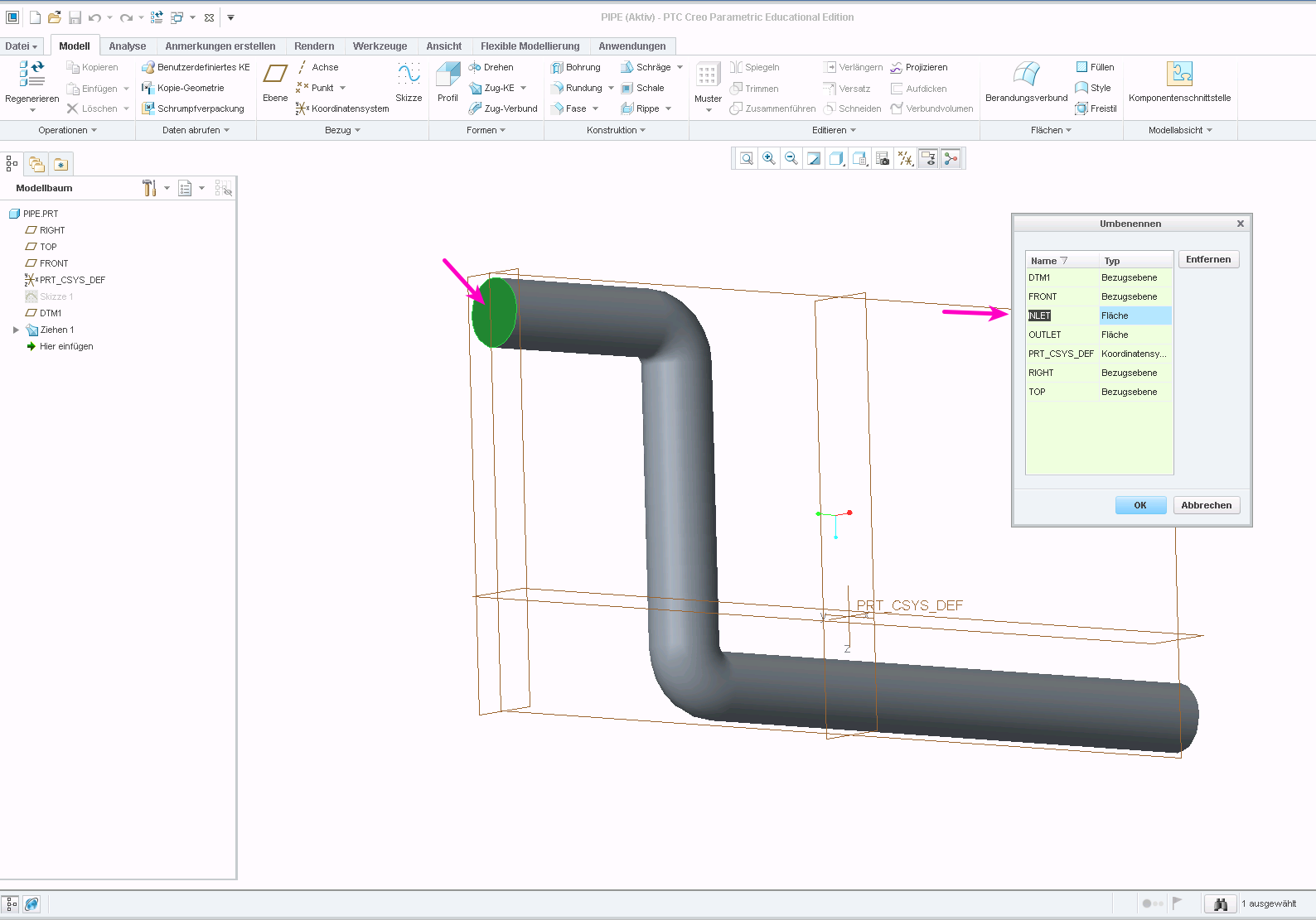
Importing CAD files for each component and its optimized parallel region meshing process using snappyHexMesh are essential for the conservative flux coupling of the different heating regions.

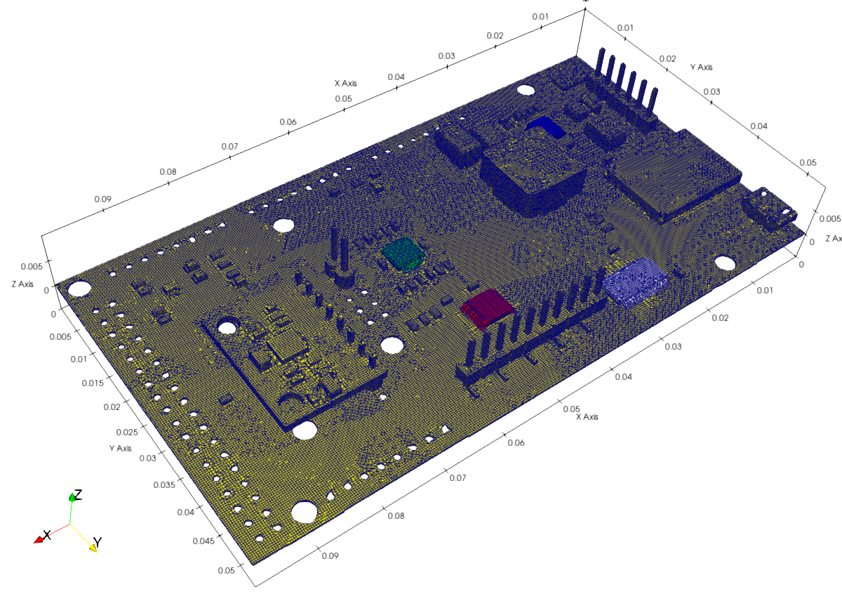
Notice that the usage of different Vias, copper wires, heat conduction layers, or other heat-related points needs to be addressed in the simulation model. Using region modeling, cell sets, and layer definitions for each component allows for the consideration of all required thermal properties.

Allowing for specially defined wildcards, CHT simulation setup is nearly automated. 

Moreover, improved heat radiation handling and optimized solver settings form the basis of stable and convergent simulations. 

Space limitations and high cost pressures increasingly lead to more complex and smaller hydraulic tanks. This results in a dramatic reduction of air separation in the tank and, consequently, an increased amount of free air in the hydraulic system.

In hydraulic systems, free air is still a technical challenge today. As long as the air is dissolved in the oil, it does not change its properties.

On the other hand, undissolved air, i.e., air bubbles, cause:

• Corrosion on pumps and controls
• Increased compressibility of hydraulic fluid can reduce the efficiency of pumps and hydraulic motors, leading to possible stuttering movements of the output member.
• Accelerated oil aging
• varnish noise
• Damage to the components (e.g. cavitation)
• etc.

Air enters the circuit during assembly, through leaks in the negative pressure zone, and as oil flows back into the reservoir. Depending on the separation capacity of the filter-tank system, the air in the tank only rises slowly and is then re-sucked by the pump.

Simulation of air-liquid devices

Silentdynamics uses InsightCAE to perform a number of simulations of dispersed gas bubbles in a degassing tank. Application of the solver twoPhaseEulerFoam enables the transient tracking of the gas phase, integral values of air at the outlets, and overall the quality of the degassing device. 

As an example, a simple degassing scenario is presented. There is one inlet and two outlets, with a weir located in the center. The oil-gas mixture flows over the weir for degassing.

 

Setting up gas-oil dispersion boundary conditions such as gas bubble size, blending coefficients, and phase properties for the simulation using twoPhaseEulerFoam could be initiated.

Using advanced solver settings within the InsightCAE framework, large time steps are enabled to manage simulations within a reasonable timeframe.

Isosurfaces of 1% gas are presented. 

---

Changing the degassing tank geometry using numerical simulation leads to a sufficient degassing process of the hydraulic oil.

When preparing geometry for numerical simulations, it is often required to mark individual surfaces in the model. These surfaces can then be used, for example, as an inlet or for applying forces and pressures in a structural simulation.

The STEP format supports named entities. The question is: how to set the names in the CAD program? And how to achieve that they are actually stored in the STEP file? In the following, these questions are answered for the software PTC Creo.

Name Surfaces

Select “File” > “Prepare” and then “Open Model Properties”, then select “Names” in the model properties dialog:

  

You can then select faces by clicking on them and enter a name in the dialog box:

Exporting Names in STEP File

If you export an STP file with the default settings, the names will not be stored in the file. You need to change the export setup for them to be kept.

Open the settings dialog via “File” > “Options”. Then navigate to “Configuration Editor”. Here, you need to add the option “intf_out_assign_names” and set it to “user_name”.

Accessing Named Entities in ISCAD

It is now possible to access faces through their assigned names, e.g., in ISCAD. Once the STEP file is imported, its sub-entities can be explored by typing Ctrl-I (see below). The named faces appear as “face_” in the hierarchy:

FreeShip software is a convenient tool for designing hulls.
The capabilities of FreeShip are essentially limited to the design of the fuselage exterior. For everything else, a real CAD system is required. There is an IGES export function for the transfer.
There is also a successor: DelftShip. The IGES export function has been removed from the free version of DelftShip and is only available in the commercial version. This is not available to me, so I cannot test it.
I would like to use the geometry in our tool ISCAD. It is based on OpenCASCADE.
The hull geometry modeled in FreeShip 2.6 looks like this:
The export to an IGES file is unremarkable and creates 40 individual faces.
The next step is the import into OpenCASCADE. However, there is a problem. OpenCASCADE (v7.2.0) reports:

Report: 40 unknown entities.

Total number of loaded entities: 41.

Nothing is displayed. Although it is reported that an import works with earlier versionshttps://forum.freecadweb.org/viewtopic.php?t=1670), the import doesn't work with the current OCC version, nor with different older versions of Salome (and OpenCASCADE). On the other hand, the import works, for example, in the commercial CAD software Creo.

Finally, a study shows that the file exported by FreeShip contains only entities of type 128 (spline surface). In addition, there is a single color definition at the beginning. At the end of the parameter block of a 128 surface (see e.g. https://wiki.eclipse.org/IGES_file_Specification#Rational_B-Spline_Surface_.28Type_128.29) are the start and end parameters (min/max U and V values) of the surface. These entries are omitted by FreeShip and for OpenCASCADE this is an error.

One workaround is to patch the IGES import of OpenCASCADE. The corresponding code is located from line 188 in the file IGESGeom/IGESGeom_ToolBSplineSurface.cxx. I removed the error message and inserted default parameter limits:

  if (!PR.ReadReal(PR.Current(), aUmin) || !PR.ReadReal(PR.Current(), aVmin)){
    //Message_Msg Msg106("XSTEP_106");
    //PR.SendFail(Msg106);
    aUmin=0.0;
    aVmin=0.0;
  }

  if (!PR.ReadReal(PR.Current(), aUmax) || !PR.ReadReal(PR.Current(), aVmax)){
    //Message_Msg Msg107("XSTEP_107");
    //PR.SendFail(Msg107);
    aUmax=1.0;
    aVmax=1.0;
  }

With these modifications, the import works: