InsightCAE is free software; you can redistribute it and/or modify it under the terms of version 2 of the GNU General Public License1 as published by the Free Software Foundation. You accept the terms of this license by distributing or using this software.
This manual is Copyright (c) 2017-2021 silentdynamics GmbH.
Permission is granted to copy, distribute and/or modify this document under the terms of the GNU Free Documentation License, Version 1.3 or any later version published by the Free Software Foundation; with no Invariant Sections, no Front-Cover Texts, and no Back-Cover Texts. A copy of the license is included in the section entitled ”GNU Free Documentation License”.
1.2About InsightCAE
InsightCAE is a framework for building automated analysis and design workflows in Computer-Aided Engineering with a preference for open source tools.
Individual open source projects often meet only subtasks in an analysis process and have very different APIs. To conduct computational tasks, a combination of several software tools is often required. In order to use open source software productive and efficient for everyday tasks, the analysis automation framework InsightCAE was created.
InsightCAE serves as a framework for the implementation of analysis procedures. The objective is to provide adapters and interfaces to the tools and simulation programs that are needed for a specific computing task.
Some common use cases are:
create a simulation app
InsightCAE’s toolkit library is used to build a simulation app. The workbench or the web interface can be used to present the parameter form to the user and display a 3D preview of the setup. The app generates a result set. InsightCAE contains a viewer to display result sets or compare data from different result sets. The simulation app can be stored in a custom library or in a python script.
assist in creation of OpenFOAM cases
InsightCAE contains a GUI (called ”Case Builder”) to build OpenFOAM cases by putting features together into an OpenFOAM case.
build parametric, script-based CAD models
InsightCAE contains an interpreter for script-based CAD models. The underlying CAD kernel is OpenCASCADE (a BREP kernel). This can utilized to produce geometry in the course of optimizations, for example.
1.3Contributors
The following people have so far contributed to InsightCAE:
Hannes Kröger (silentdynamics GmbH)
Johann Turnow (silentdynamics GmbH)
If you want to get involved in the development, please feel invited to do so! We greatly appreciate any contribution and we would very much like to add you to the above list.
If you made some modification or addition to the code, which you would like to be merged into the main development line, please consider to send us a pull request2 .
1.4Features and Highlights
InsightCAE’s objective is to create automated analysis workflows. The high level API resides in the core ”toolkit” library. Automated workflows usually involve different external programs and utilities. For the realization of automated workflows, it is sometimes required, to create add-ons to these external programs. Thus InsightCAE is also a container for add-ons to other programs.
InsightCAD script-based, fully parametric CAD
OpenCASCADE geometry kernel
assemblies, constraint-based sketches, part library, drawing export
Pre- & Postprocessing tool (OpenFOAM Case Builder)
analysis workflow automation tools (GUI)
1.5Reading this Manual
1.6Recommendations for Working with Shell-based Tools in Linux
Sometimes it is necessary to execute tools in a bash shell, e.g. because no GUI for it is available. And often it is easier to keep an overview in graphical file manager. Having a console window open together with a file manager window at the same time is an obvious solution but to do so for many cases at a time may easily confuse the desktop.
Here are two useful hints to solve this issue:
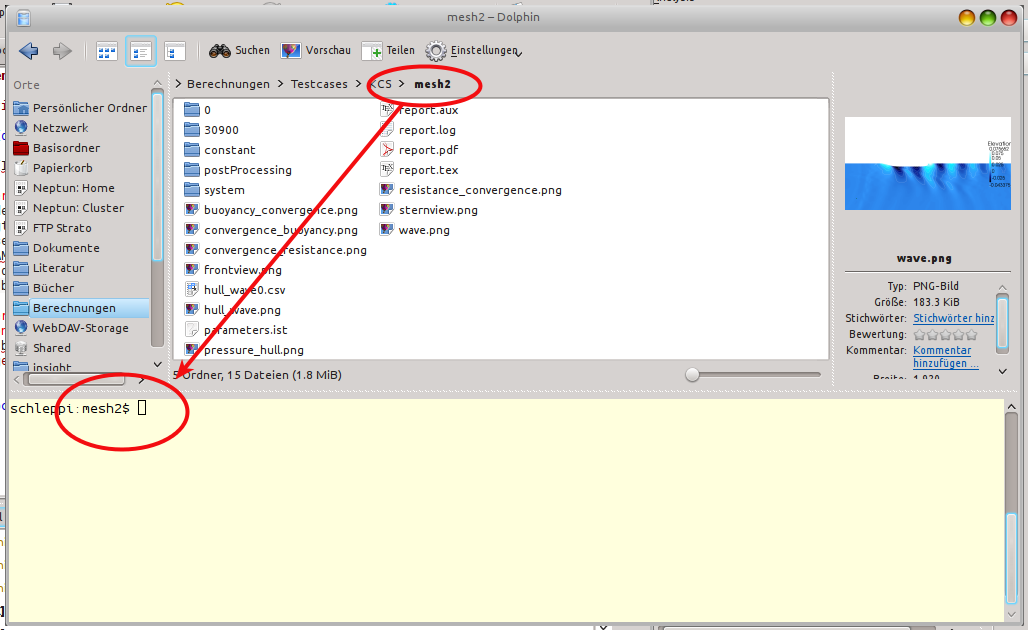
The KDE file manager dolphin offers the possibility to display a console in the lower half of the window (figure 1). The working directory is synchronized with the directory shown in the graphical window by injection of cd commands. Vice versa, when the working directory is changed in the shell, the graphical display is updated as
well.
Figure 1:Dolphin file manager with embedded terminal
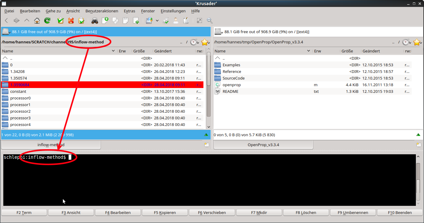
There is a Norton-Commander-like file manager named krusader (figure 2). It offers the same functionality regarding the embedded terminal but a more flexible way of displaying multiple folders. In addition to the two list view on the left and right, multiple tabs for folders can be added in each list view. And there is also a rich interface to define custom
commands and file associations.
Figure 2:Krusader file manager with embedded terminal
Beyond the web resources above, silentdynamics GmbH offers commercial support3 for professional users of InsightCAE. Automated analyses according to customer needs and specifications are implemented by creating new specialized modules for Insight CAE. Typical support contracts include also user training and continuous customization and updating of
InsightCAE and its add-ons.
3Obtaining InsightCAE
3.1Installation using Linux Package Manager
We provide binary installation packages for Ubuntu-based Linux distributions. We specifically support the latest Ubuntu LTS distibution.
The packages are held in our repository. To install them, first add the silentdynamics apt repository and the associated key by executing:
Then, you can install the community-edition package by executing
1$sudo apt-get install insightcae
Continue with preparing the environment according to section 3.4
Note: for customers who receive supported, tailored simulation apps from silentdynamics, these apps are bundled into add-ons and the add-ons are included in a tailored installation package. For each customer, a separate package repository is maintained (with a unique URL, different from the one above). This needs to be included additionally to the one above. These packages are then named insighcae-<customername> and the install command changes to:
1$sudo apt-get install insightcae-<customername>
Note: besides the standard repository at http://downloads.silentdynamics.de/ubuntu which includes the package built from the ”master” branch in the git source code version management system, silentdynamics provides a second package repository with a development package built form the branch ”next-release”. To use this repository, just switch the URL in the instructions above to http://downloads.silentdynamics.de/ubuntu_dev.
3.2Installation on Windows
Our software as well as OpenFOAM and Code_Aster are currently pure Linux software. However, it can also be run under Windows 10 (64 bit only) or later with the help of the ”Linux Subsystem for Windows” (WSL). Virtualization is not used. The processes share the memory with the Windows processes and the files are stored in the Windows file system.
Graphical output from the WSL environment has turned out to be error-prone and poor, thus the software is split into a frontend part, which runs natively in Windows and a backend part which controls the simulation solvers and runs in the WSL environment. The communication between both is over the network stack.
For the comfortable installation of InsightCAE and OpenFOAM under Windows we provide an installer. The installer for the stable version (master branch in the git repository) can be found in this directory:
The installers for the different versions X.Y.Z are named in the form
InsightCAEInstaller-X.Y.Z.exe
Note: for customers who receive supported, tailored simulation apps from silentdynamics, the installer is downloaded from the customers dedicated repository URL instead of the one above.
Download the latest EXE file from this link and execute it:
It will activate the Windows subsystem for Linux, if it is not already activated
The installer bundles the necessary third party programs (ParaView, gnuplot, MiKTeX, Putty)
Note: it is required that the python runtime library (python36.dll) is in the library search path (PATH environment variable). There is an option in the python installer which should be enabled by the user (it is disabled by default).
If this is missed, the PATH variable needs to be manually edited after the installation.
Please note:
For the installation, administrator rights are required
Usage Appropriate start menu entries are created.
To complete the setup, perform a system reboot and launch the InsightCAE ”Workbench” from the start menu.
Upon the first launch, two things need to be completed:
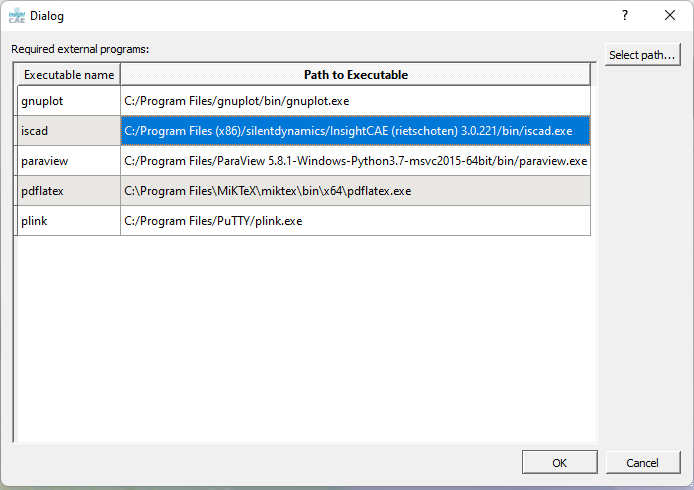
Set paths to commonly required executables.
The executables are searched in the executable search path defined by the system. Some will not be found since their location is not included in the executable search path environment variable PATH. If some of the required executables are not found, the configuration dialog shown in figure 3 is brought up. Click on a row, where no ”Path to executable” is
printed and click on ”Select path...”. In the dialog box, find the appropriate executable and click ”ok”. Repeat this for every executable, which was not found.
The presence and the version of the WSL backend is checked.
The installer package includes a WSL image matching the version of the installer. This image is installed, when the installation is performed. Thus this check should be silently successful.
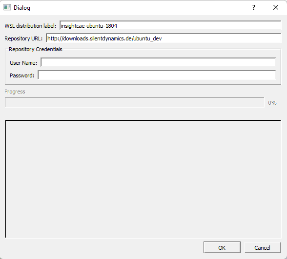
If there is no WSL existing, a message appears and the user should select ”Create” to create one. The form as shown in figure 4 should appear.
The URL should be properly preset according from which source the installer was downloaded. For support customers, it is important to enter their credentials into the appropriate fields.
When everything is set, click the button ”Ok”. Then the image is downloaded from the server and installed. The image is approximately 1.5GB so the download takes some time and also the unpacking takes several minutes. When the creation is done, the creation dialog is closed and the workbench GUI is shown.
Figure 3:Configuration dialog to set the paths to commonly used third party executables
Figure 4:Create WSL backend form
Updating To update to a newer version, just download the newer installer from the location described above and execute it.
Only the last two components (“WSL Distribution” and “InsightCAE Windows Client”) needs to be checked in the installation wizard. If the third party tools were already installed, they should be skipped.
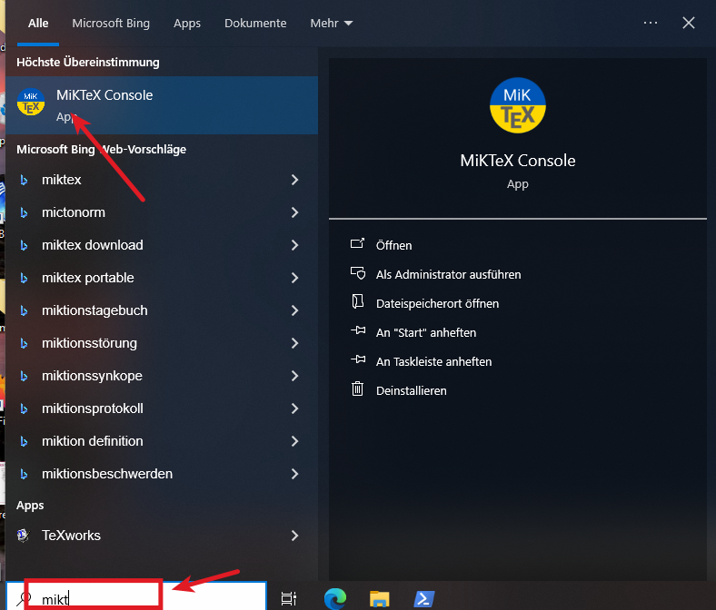
Updating Dependencies – MikTeX MikTeX is independent from InsightCAE and used by InsightCAE for generating PDF reports and also for rendering charts. Sometimes it might be required to update it. This is done using the following steps:
Open the MikTeX console, e.g. by typing the Windows key and then the command ”miktex console” until the icon appears. See figure 5.
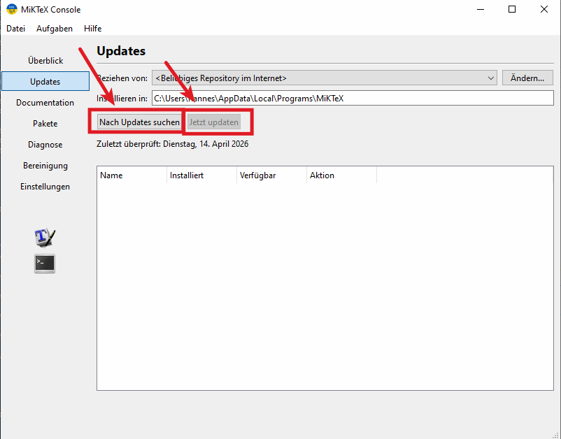
Change to the tab ”Updates”. First click on ”Search for Updates”. When updates are found, click on ”Update Now” and follow the instructions. See figure 6.
Figure 5:Updating MikTeX, finding the MikTeX console
Figure 6:Updating MikTeX, executing the update
3.3Building from Sources
3.3.1Getting the Source Code
The source code of InsightCAE is hosted at Github. Cloning a working copy constitutes the best way to get updates and the latest bug fixes.
Alternatively, you can download snapshot archives from github, if you don’t want to bother with a git client. In this case, just replace the cloning step below with unpacking the archive.
First, get the the sources by cloning the git repository:
The InsightCAE project depends on a number of other projects. Some of the dependencies are optional and only required, if certain features are enabled. The dependencies are listed in table 1.
Project
tested version
required for
Armadillo
9.800.4
(always)
Gnu Scientific Library
2.6
(always)
Boost
1.65.1
(always)
VTK
9
(always)
Python (Lib)
3.6
(always)
OpenCASCADE
7.4
(always)
DXFlib
3.7.5
(always)
libpoppler
0.86
(always)
Qt
5.15
for GUIs
Gmsh
4.8
only for analyses with tet/tri meshing
Wt toolkit
4.1
only for client/server execution
OpenFOAM
ESI1806, 4.1 extend
only for OpenFOAM based analyses
Code_Aster
14
only for FEM analyses
SWIG
4
only for python bindings
Table 1:Required dependencies for building InsightCAE
3.3.3Building
CMake is utilized for managing the build. The preferred way is to build the software out of source in a separate build directory. Create a build directory, then configure the build using e.g. ccmake and finally build using make:
In the CMake GUI, you may need to change paths or adapt settings. Please refer to the CMake documentation4 on how to use CMake. The biggest difficulty will probably be, to provide all the software packages, on which InsightCAE depends.
The final step in CMake is, to generate the Makefiles. Once this is done without errors, start the compilation of the project by executing:
1$make
To work with InsightCAE, some environment variables are needed to be set up. A script is provided therefore. It can be parsed e.g. in your ~/.bashrc script by adding to the end:
1source/path/to/insight/bin/insight_setenv.sh
3.4Setting up the Environment
To set up the environment variables and search paths required by the InsightCAE components, a script needs to be parsed. This is conveniently added to the shell startup script file ~/.bashrc. Add the following line to the beginning of the ~/.bashrc file:
1source/opt/insightcae/bin/insight_setenv.sh
Note that the default contents of this file differs between linux distributions. Sometimes it contains statements which prematurely end its evaluation for non-interactive shells. This
4Overview of the Project InsightCAE
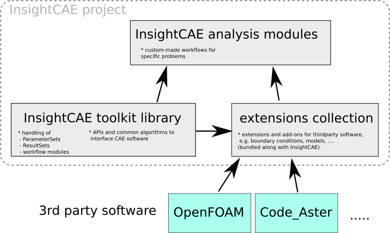
4.1Concept and Parts of the Project
The InsightCAE builds on top of available open-source engineering analysis tools (though closed-source tools could be used as well). The most used tool by far is the CFD software OpenFOAM.
For certain tasks, custom extensions to these tools are required. InsightCAE contains a selection of extensions, which are included in the distribution packages, when these are created.
The core of the project is the toolkit library. It contains the implementation of core classes in workflow management as the parameter set storage and tools and result set storage classes and handling tools. The toolkit library also maintains a list of available analysis modules, which is dynamically extensible by loadable add-ons.
Finally, on top of the toolkit library, custom analysis modules can be created. The InsightCAE base distribution contains a number of generic analysis modules as the ”Numerical Wind Tunnel” module and some generic test case analyses like flat plate, channel flow, pipe flow and so on. These might serve as examples for custom implementations.
Figure 7:Structure of the InsightCAE project
4.2Terms and Defintions
Simulation App, Analysis InsightCAE bundles tools to create automated simulation procedures. These procedures can be written in Python or C++. The term analysis, workflow module or Simulation App is used for such a procedure.
Actually, an analysis is like a function in programming: it gets input parameters, executed some actions (e.g. a numeric simulation) and returns a results data structure.
InsightCAE provides a GUI to edit the parameter sets and also tools to work with the result sets. E.g. convert the result set into a PDF report.
Parameter Set The analysis modules need input data, i.e. parameters. All parameters for a module are grouped together in a parameter set. Parameter sets are stored in XML files in human readable format (extension *.ist). They can also be edited in a GUI editor (application workbench).
Many analysis modules need external files (like CAD data in STL or any other format). These files can simply be referred in a parameter set by their relative path (relative to the *.ist-file containing the reference) or absolute path. It is also possible to embed the external files into the XML file in an base64-encoded form. This simplifies transfer of analysis setup from one computer to another, e.g. for remote execution.
Result Set The result of an analysis is returned in a result set. This is a hierarchical data structure which contains nodes like scalar values, charts, contour plots, images, tables or similar entities. It can be stored on disk in XML format. There is also a renderer which converts a result set into a PDF report.
Case Element The setup of CFD-runs is put together from a number of so-called case elements. Each case element represents some functional feature. It might be a boundary condition or a turbulence model or something similar. A case element is not necessarily associated with a certain configuration file but can modify multiple configuration files of a CFD
case configuration.
There is also an editor for composing OpenFOAM cases from the available case elements: the OpenFOAM Case Builder.
Solver extensions
OpenFOAM Case Builder
Workbench
Part I Workflow Automation
5Simulation Apps
5.1Explanation of Building Bricks
5.1.1Input: Parameter Sets
Parameter sets are a hierarchical collection of parameters. Parameters can be of different type, see table 2 for a list.
A parameter set constitutes the full input data set for an analysis.
Beyond these primitive parameter types, there can be compounds, namely:
subset
a subdirectory in a parameter set
selectablesubset
a subset that switches its content based on a selection parameter
array
an array of either a compound parameter or a primitve parameter
Throughout this manual and also e.g. in the command line parameters, the parameters are commonly specified in a file path-like format, where subsections are separated by slashes. For example, the parameter evaluateonly in the subsection run is meant by the expression run/evaluateonly.
For arrays elements, the index of the element is inserted after the array parameter name. For example, the parameter mesh/refinementZones/0/lx refers to the parameter lx inside the first array element of the array of subsections refinementZones in the subsection mesh.
Type
Description
double
a scalar floating point value
int
an integer value
bool
a boolean value
vector
a 3-tuple of doubles
string
a simple text
selection
a selection from a predefined set
path
a file path, relative to the input file
matrix
a matrix with arbitrary number of rows and cols
doublerange
an array of double values
Table 2:Available primitive parameter types in a parameter set
5.1.2Output: Results Sets
The output of an analysis is stored in a result set. It may contain elements like charts, images, tables, number etc. A result set can be saved to a XML file and/or rendered into a PDF report.
5.1.3Analyses: the Simulation Procedure
The procedure of a simulation is contained in a so-called analyses or workflow module. You may think of it as an app for executing a certain type of simulation. It is essentially a program. Oftentimes, people create scripts or macros for speeding up their simulation workflows. The InsightCAE workflow modules serve a similar purpose, though the intention is to fully cover the whole simulation including all pre and post processing steps.
There is a GUI available which provides an editor for the input parameter set (see section 5.2.1). The GUI is also capable of displaying a 3D preview of the involved geometry and other elements, which are displayable. The analysis module is responsible of creating the 3D preview elements. Creation of the preview is optional and not every analysis module produces a preview.
The GUI also includes a viewer for the result set. From that viewer, the reports may be exported.
InsightCAE holds a runtime-extensible list of available analyses. This list can be extended at run time either by providing shared libraries containing more analysis modules or by python scripts.
The analyses can be programmed essentially in C++ or in Python. InsightCAE is essentially written in C++. Python wrappers for the relevant functions and objects are created using SWIG. So the API can also be accessed from Python.
If a new analysis shall be created, this parameter editing and result viewing infrastructure is easily reusable:
The new analysis module just needs to provide the parameter set layout by returning the default parameter set (a parameter set filled with suitable default values),
it has to provide a function for executing the analysis.
This function needs to return a result set.
The analysis modules may group themselves into categories. This is used in the initial analysis creation dialog in the GUI.
Python Script A python based analysis comprises a single dedicated python script file. The InsightCAE functions are included by an initial statement like from Insight.toolkit import *.
This script needs to define three standalone functions:
category()
This functions returns a plain string with the category of the analysis. Multiple hierarchy levels are supported and have to be separated by slashes.
defaultParameters()
This function shall return an object of type ParameterSet, containing the default values of all the needed parameters. The user cannot add or delete parameters, just modify their values. So this defines the layout.
executeAnalysis(parameters, workdir)
This function finally runs the simulation. It gets an object of type ParameterSet, containing all the input parameters and the string workdir, which contains the execution directory.
Upon loading, the InsightCAE base library searches in
$INSIGHT_GLOBALSHAREDDIRS/python_modules and
$INSIGHT_USERSHAREDDIRS/python_modules
for files named *.py. Each of these files will be loaded and their defined analyses will become available in the GUI and all other InsightCAE tools.
C++ In C++, a new analysis is derived from the common base class Analysis. The necessary functions have to be overridden. The new analysis should be put into a dedicated shared library.
Upon loading, the InsightCAE base library searches in
$INSIGHT_GLOBALSHAREDDIRS/modules.d and
$INSIGHT_USERSHAREDDIRS/modules.d
for files named *.module. Each of these files has to contain a statement library <FILENAME>, where FILENAME is the name of the shared library file. These libraries will all be loaded and their defined analyses will become available in the GUI and all other InsightCAE tools.
5.2Usage
5.2.1GUI: workbench
The GUI for editing analysis parameters, run analyses and monitor their progress and to review the result sets is called workbench.
It can be started from the command line by executing
1$workbench
or from the global application menu.
The workbench can open and handle multiple analyses at a time. For each analysis, a sub window is opened (analysis form).
An analysis can either be created from scratch (see “Creating a New Analysis”) or by opening an existing analysis input file (select in the menu).
The analysis form has three tabs. From left to right: the input parameter edit tab, the progress display tab and the result viewer tab.
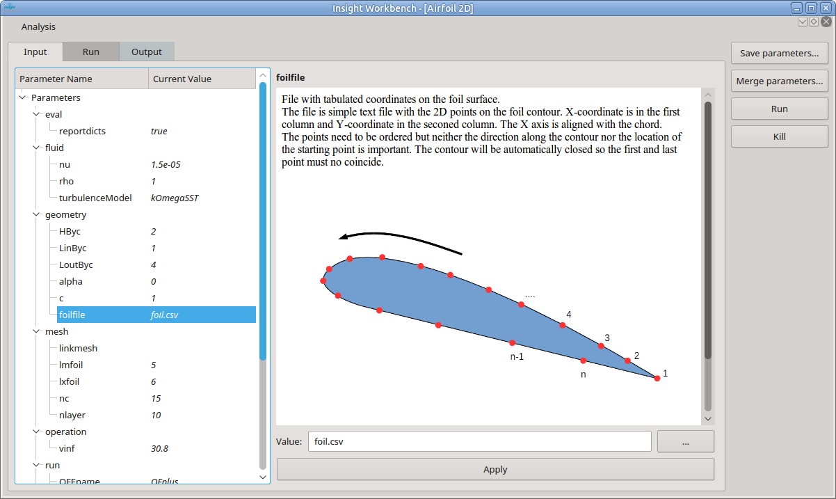
Editing the Input Parameters The parameter input tab is shown in figure 9. On the left, there is a tree view showing all the available parameters of the analysis. The font display style of the parameter entry denotes the importance of the parameter:
highlighted yellow background: these parameters have no reasonable default values and need to be changed for every case. The displayed default values are only chosen to demonstrate some functional value, e.g. for speeds or rpms. But for parameters like file names, for example, there is no reasonable default at all.
normal black text color: these parameters have reasonable default values, with which an analysis can be started. Though it is quite normal, that these parameters might need to be adapted from case to case.
dimmed gray text color: these parameters should normally be left at their default values. But it for rather rare special cases, it might become necessary to adapt them.
The parameters can be selected my mouse click and edited (see “Modifying a Parameter”).
Some analyses (this is optional) support a 3D preview of the configured case. When an analysis is loaded, which supports 3D preview, a 3D view and a 3D element tree appears right of the parameter edit column. All views in the Input tab are shown in a horizontal splitter and their width can be adapted by dragging the splitter handle between them. It is also possible to hide the 3D preview widgets by collapsing their width to zero using the splitter handle (This might also occur
accidentally). The collapsing can be undone by locating the splitter handle of the collapsed widget and dragging it back to some non-zero width. The layout of the splitter is saved on program exit and restored on the next start.
Saving Parameters Once all parameters are edited, the parameter set can be saved to a file. Very often, external files are referenced from a parameter set. Since it is also often necessary, to relocate parameter sets from one computer to another or between directories, InsightCAE parameter sets provide some special features which shall simplify relocation
of parameter sets:
file paths are always stored as relative paths inside the parameter set file.
Even if the workbench editor displays an absolute path, the paths are made relative to the saving location of the parameter set file. It is still possible to insert absolute paths into a parameter set file. But when it is loaded and saved again, these will be made relative.
If a parameter set is moved around together with the files it references, they will be found, as long as they remain in the same relative location, e.g. side by side with the parameter file or in a sub directory.
external files can be embedded into the parameter file.
This is the preferred option, when parameter files shall be moved across computers. Upon saving, the files will be base-64 encoded (not compressed) and stored in the XML file. When the analysis is run, the files are extracted to a temporary location. The extraction is aware of the case, that different files with the same name might exist in different directories and extracts them to different locations. By default, the files are extracted to the system temporary location. When the
InsightCAE application, which triggered the extraction of the parameter, exits, the files are deleted again from the temporary location. Note that this might not be achieved, if the application crashes.
Packing of external files can be enabled by checking or by checking the appropriate option in the ”Save Parameters” dialog. Once, a parameter file was saved as packed or unpacked, the selection state is saved and used for all subsequent save operations.
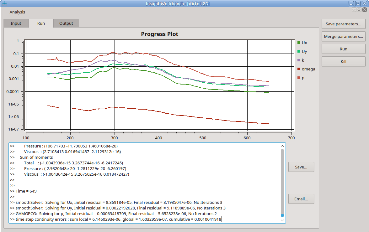
Running the Analysis With a properly edited parameter set, the analysis run can be started. This is achieved by clicking on the button ”Run” on the right side or by selecting in the menu. This analysis form switches automatically to the ”Run” tab (see figure 10). In the lower half, the log message are displayed. Sometimes, errors in an external program occur and are not correctly reported. It is therefore a good practice to watch the log messages for errors or warnings.
When the simulation solver runs, InsightCAE shows progress variables graphically. The plots are shown above the log widget. The number and meaning of the progress variables depend on the analysis conducted.
Especially for OpenFOAM-bases analyses, a number of quantities are extracted from solver output and forwarded to the GUI as progress variables:
continuity errors
equation residuals
forces
moments
execution time (per timestep)
Cancel a Simulation To cancel a simulation run, click on the button ”Kill” on the right side or by select in the menu.
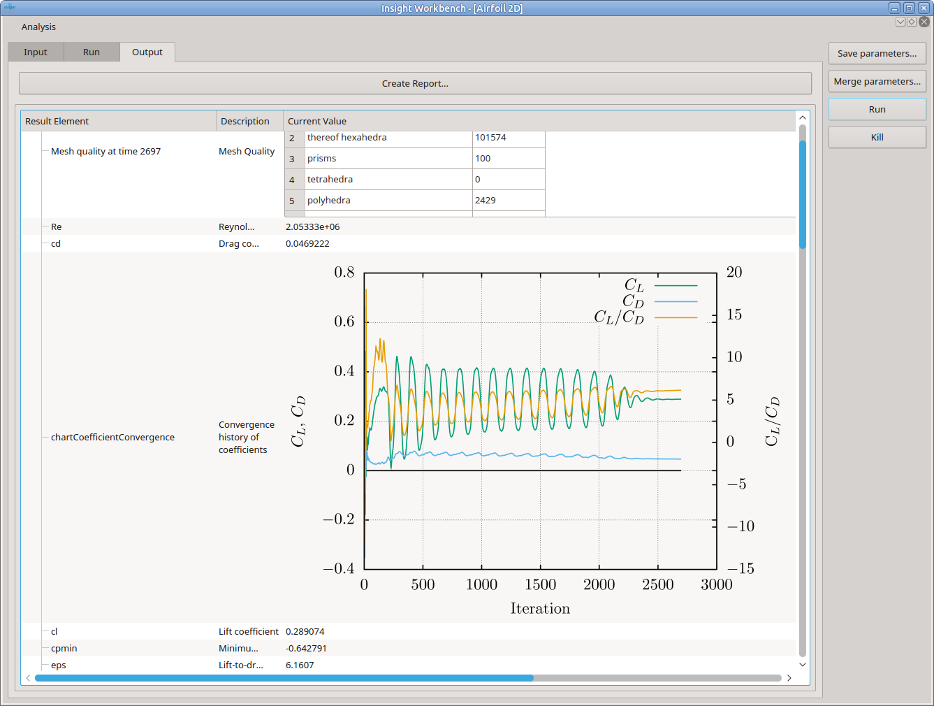
Viewing the Results Once the simulation run is finished (that means that the solver has finished and that all post processing steps are done), a result set is created and loaded into the workbench. It is displayed in the ”output” tab (see figure 11). The result set can be rendered into
a report (see “Rendering Results into a Report”).
Rendering Results into a Report
Modifying a Parameter
Creating a New Analysis A new analysis is created by selecting in the menu . Then a new dialog appears, in which the list of available analyses is displayed (figure 8). The
required analysis should be selected and confirmed by clicking ”Ok”.
Figure 8:Dialog for selection of the type of a new analysis
Figure 9:Parameter editing tab of the workbench
Figure 10:Solution progress tab of the workbench
Figure 11:Result explorer tab of the workbench
5.2.2Special Features for OpenFOAM-based Simulation Apps
Simulation apps which are based on an OpenFOAM simulation provide some special features and also some implicit behavior and conventions which is documented in this section.
Restart Behavior OpenFOAM-based simulations often run for a long time. It frequently appears that the simulation procedure is interrupted, either accidentally or intentional, and needs to be restarted.
There is no explicit function for a restart. It happens implicitly, when the analysis is re-launched in an existing working directory and some preconditions are met.
Depending on the state of the data, the behavior will be as follows:
if a mesh exists (in folder ”constant/polyMesh/”) and a time directory exists (e.g. ”0/”): it is assumed that the case is ready for execution and the solver will be restarted,
if only the mesh exists (”constant/polyMesh/”) and no time directory: mesh creation will be skipped. But all the dictionaries in constant/ and system/ and field files in the initial time directory will be recreated.
Depending on where the interruption happened, the state might be inconsistent and invalid behavior might result. For example:
the interruption appeared within a meshing procedure which includes intermediate meshes ⇒ a mesh will be present but invalid
the interruption appeared during the field initialization ⇒ a time directory is present but the fields are invalid,
the interruption appeared during writing of a time directory ⇒ a time directory is present but invalid and the solver restart will fail.
If you are unsure about the validity of the case data, please consider to clean the case directory first and restart everything from the beginning (see 5.2.2.0).
Cleaning the Case Directory When an OpenFOAM-based simulation run was performed, a number of directories and files are created in the working directory. If another run shall be performed and no restart is desired, then these directories and files need to be removed first. For this task, there is the standalone tool isofCleanCase, see section 7.4.
This tool can be launched in the selected workspace directory from within the GUI via the button ”Clean” on the right side of the analysis form. Please see section 7.4 for details on the usage.
In some OpenFOAM-based simulation apps, auxiliary OpenFOAM case are created in subdirectories of the workspace directory. Currently, these can only be deleted or cleaned manually via a file manager and the command line tool isofCleanCase.
Performing only the Evaluation without Running the Solver This is needed, if the solver was manually restarted, e.g. after manual changes of the numerical settings became necessary due to stability problems and ran until completion in the case directory which the corresponding InsightCAE simulation app has
created.
It is then possible to execute only the evaluation part of the simulation app alone. This will not do any modifications to the simulation setup and it will not start any solver. To do this, the following is needed:
in the parameter set, set the switch run/evaluateonly to true,
set the working directory to the existing case directory, where the case was created (this will be done automatically, if an existing input file was opened),
then start the simulation by clicking the ”Run” button.
Please note, that all parameters in the input file are assumed to match the simulation setup. No checks are done and there is no possibility for the Simulation app to restore them from an existing simulation folder. Thus it is up to the user to ensure validity.
Launching Graphical Postprocessor ParaView To inspect the results of a OpenFOAM simulation beyond the figure which the InsightCAE simulation extracts automatically from the simulation case, the independent graphical postprocessor Paraview can be used.
It can be launched from the command line using a script as explained in 7.5.1.0.
Alternatively, this can be done also from the workbench. On the right border of the analysis form, there is a button labelled ”ParaView”. For OpenFOAM-based simulation apps, this is enabled. Once it is pressed, Paraview will be launched in the selected working directory. If a local run is configured, it will just read the case from the selected working directory. If a remote run is selected, a client-server pair will be launched and the connection to the remote side is set up via SSH
tunnels.
5.2.3Console on Headless Computers: analyze
It is possible to launch an analysis from an existing input file (*.ist) without the graphical user interface in a batch mode. This is useful to integrate InsightCAE into workflows with other third-party software. The input file can be saved from the workbench (see 5.2.1.0) or created by a script or with any text editor.
To launch a simulation in batch mode, the executable analyze is available. It can be launched like this from the command line:
1$analyze inputfile.ist
The executable understands additional options. These are explanined in the following paragraphs.
Changing parameters The values of parameters in the input file can be overridden from the command line by specifying an arbitrary number of the following parameters:
The argument arg for all these options has the form: path:value. The path is the file path-like specification of the parameter (see 5.1.1) and the value is appended to the name, separated by a colon. If any spaces are inside the value, e.g. when strings or path names are to be specified, then the entire arg should be set in
qoutes at the command line. For example:
General Behaviour The simulation working directory can be set explicitly by the parameter --workdir (short -w). The default is to use the current directory as the working directory.
The finally applied input parameter set is optionally saved to a file, when the file is specified with the parameter --savecfg (short -c).
5.3Available Simulation Workflows
5.3.1Numerical Wind Tunnel
5.3.2Internal Pressure Loss
6Working with Result Sets
The simulation apps produce result sets as output. These are collections of result elements. Result elements can be for example:
Plain values: scalar or vector
Matrices
Charts
Images
Files
Tables
Result sets can be
stored in a file (extension *.isr),
displayed with a viewer program. A viewer is embedded into the workbench (tab ”output”) and a standalone viewer is available with the program isResultTools
or rendered into a PDF report.
In addition, with the isResultTool, comparisons between multiple result sets or extraction of selected elements can be done.
Rendering of a Result Set Result sets are displayed in the ”output” tab of the workbench. When there are results displayed, those can be rendered or saved into an ISR file by selecting
Whether a PDF report is rendered or a ISR file is written, depends on the file extension which is entered in the file dialog.
A report can also be rendered from a ISR file on disk. Therefore the executable isResultTool exists. Once the program is started, select in the menu and select the ISR file in the file selection dialog. The result elements are then shown in the tree view on the left side of the window (12b). To render the result elements into a PDF, select in the menu and enter a file path to the desired output PDF file.
Optionally, some result set elements can be omitted from the PDF rendering by applying filters, see 6.0.0.0.
Figure 12:Main window of the isResultTool. a) bottom left: filters to be applied to the currently loaded result set, b) top left: content directory of the loaded result set (with the filters applied), c) right side: details of the result element that is selected in the top left tree view.
Alternatively, the tool isResultTool can be executed with the command line argument --render:
1$isResultTool --render savedResultset.isr
Applying Filters during Rendering A set of filters can be defined to render a report with some result elements excluded. A filter is just a path-like text which represents the location of the result element in the result set hierarchy. The concept is very similar to the specification of parameters, see section 5.1.1 above. Every result element, where the label path matches one of the filter expressions, is excluded. The filter expressions, which are already defined, are shown in the list in the bottom left corner of the Result Set Viewer window, see figure 12a. The result set content directory, which is displayed in figure 12b, shows the result set contents with all filters already applied.
To add filter expressions, click on the button ”Add...”. The result element paths to filter out can be directly typed into the text field, one per line. Instead of typing, result elements can be select from the full content of the result set after clicking the ”...” button.
By default, a direct match of the entered text with the result element path is required. Alternatively, the text entered in the input field can be treated as a regular expression56 . If a regular expression
was entered and shall be treated as such, the selection below the input field has to be changed to ”regular expression”.
Once a set of filter expressions is defined, it can saved to a file by selecting .
Vice versa, a previously saved set of filter expressions can be loaded by .
When the a report is rendered or saved into a ISR file, there is a switch on the bottom of the file dialog (”Save filtered result set”). This is by default checked. If this is unchecked, the filter is skipped and the full report is rendered or saved.
7Supporting Simulations with OpenFOAM
7.1Case Setup GUI: isofCaseBuilder
7.2Execution Monitor GUI: isofExecutionManager
7.3Tabular Output Data Plot: isofPlotTabular
7.4Clean OpenFOAM Case Directories: isofCleanCase
7.5Common Tasks in the Context of OpenFOAM Simulations
7.5.1Controlling and Checking Running OpenFOAM Case Which Were Generated by InsightCAE
OpenFOAM cases which were generated by InsightCAE are enhanced with a number of additional features. These are utilized by the workbench frontend but can also be used to modify cases manually.
Trigger Output Independently from the Configured Output Interval The solver monitors the files in its case directory. If it finds a file named wnow, immediate output is triggered and this signal file is removed by the solver.
This feature can be used to inspect the solution at any time while the solver is running using Paraview.
The file can e.g. created from the terminal:
1$touch wnow
Note: you might need to change to working directory to the case directory first.
Trigger Immediate Output and Stop Solver Afterwards Without Raising an Error The solver monitors the files in its case directory. If it finds a file named wnowandstop, immediate output is triggered, this signal file is removed by the solver
and the solvers.
This feature can be used e.g. to gracefully and a solver run which is converged and the convergence is recognized by the user but not yet by the convergence monitoring feature of InsightCAE.
The file can e.g. created from the terminal:
1$touch wnowandstop
Note: you might need to change to working directory to the case directory first.
Inspecting a Running Case Using Paraview Some of the relevant numerical figures of a case are displayed in live updated charts in the GUI. But it is a very good habit to check the mesh and also the solution as soon as possible and well before valuable computing resource are wasted to compute inadequate solutions on bad meshes. If
problems with the mesh or the solutions become obvious, it is possible to stop the analysis (e.g. by the ”Kill” button in the workbench or by pressing CTRL+C in the terminal, where the analyze command line tool is running) and revise the settings.
The OpenFOAM cases can be loaded into Paraview as soon as they were created by one of the InsightCAE modules. It is perfectly possible to do this while the solver is running. It is also possible to trigger extra output if it is not yet available (see first paragraph of this section).
When output7 is there, Paravie w is best launched by InsightCAE’s wrapper script isPV.py:
1$isPV.py
Note: you might need to change to working directory to the case directory first.
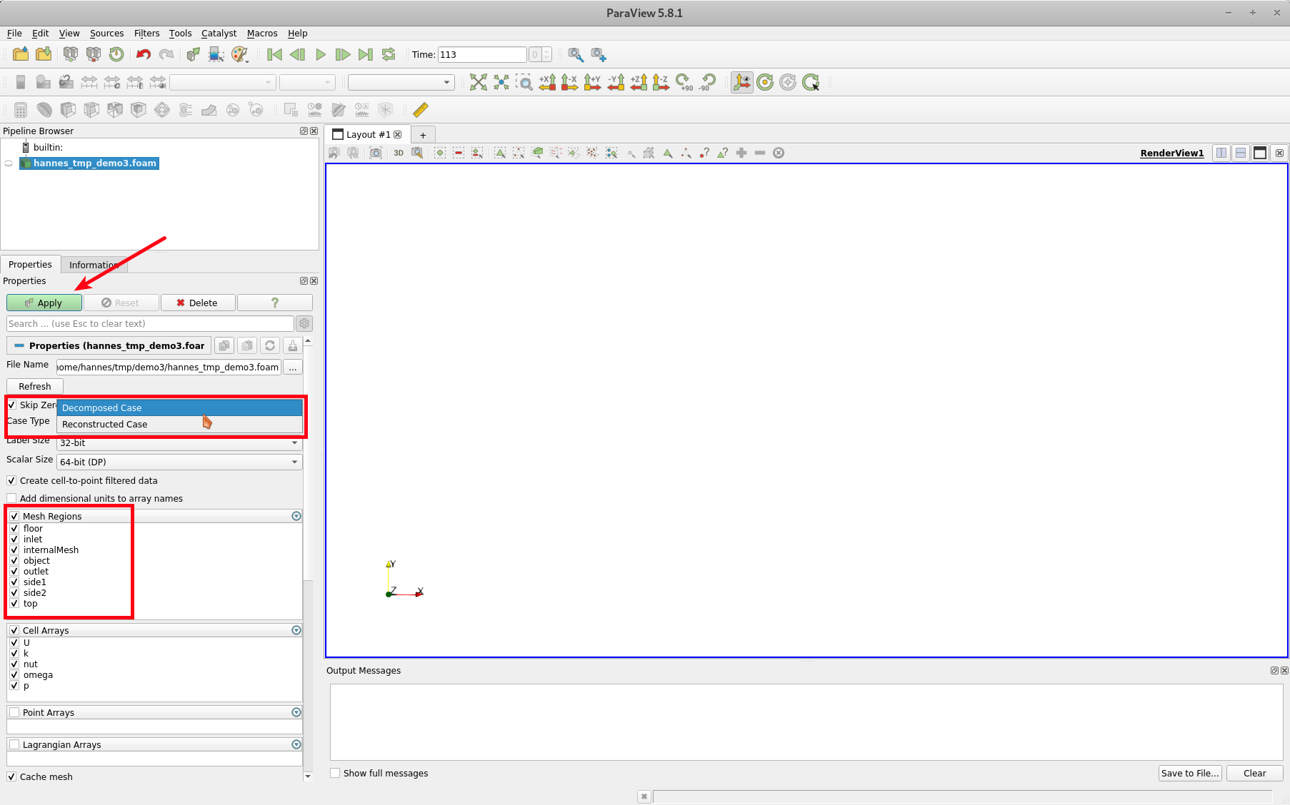
The wrapper automatically inserts the OpenFOAM case reader source into Paraviews’ visualization pipeline. You should consider the following settings:
Select at least all the mesh regions, which you would like to inspect. You can later filter out subsets of mesh regions. So it is ok, to select all.
Select the case type: either
”Reconstructed Case”, if you performed a serial run or if the output has been already reconstructed from the processor directories (usually done for the last time step during the evaluation step)
”Decomposed Case”, if you want to monitor a parallel run.
When all settings are right, click on ”Apply”.
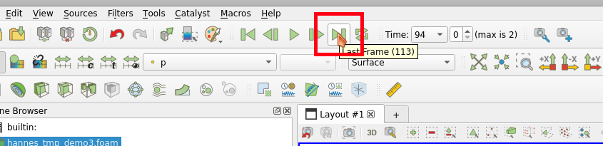
Next, jump to the latest time step:
Now, the scene can be set up using all the Paraview filters8 .
Often, fields on boundary regions (e.g. walls) are of interest. These can be extracted using the ”Extract Block” filter. To apply this filter, select from the menu . Make sure that the OpenFOAM case source is selected in the pipeline browser when the filter is added. When all the boundaries of interest are selected, click on ”Apply”.
7.5.2Meshing
Extraction of Feature Edges from STL Geometries Features edges can be extracted automatically from STLs. They are usually found by looking at the angle between neighbouring triangular facets. This methods is usually automatically applied either in snapphyHexMesh itself or within InsightCAE’s workflows. This method works nicely for edges between planar
surfaces. Though it fails e.g. for rounded edges like leading and trailing edges of propellers and foils. In such cases, it is required to extract feature edges manually and feed them into the meshing process.
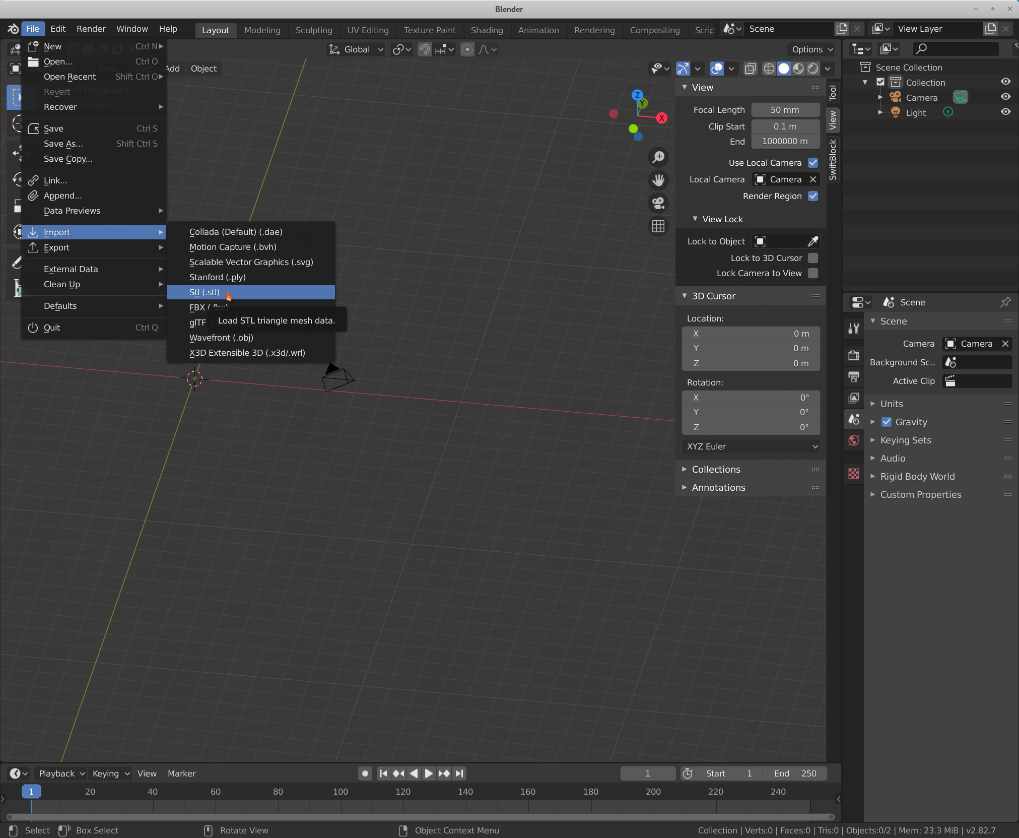
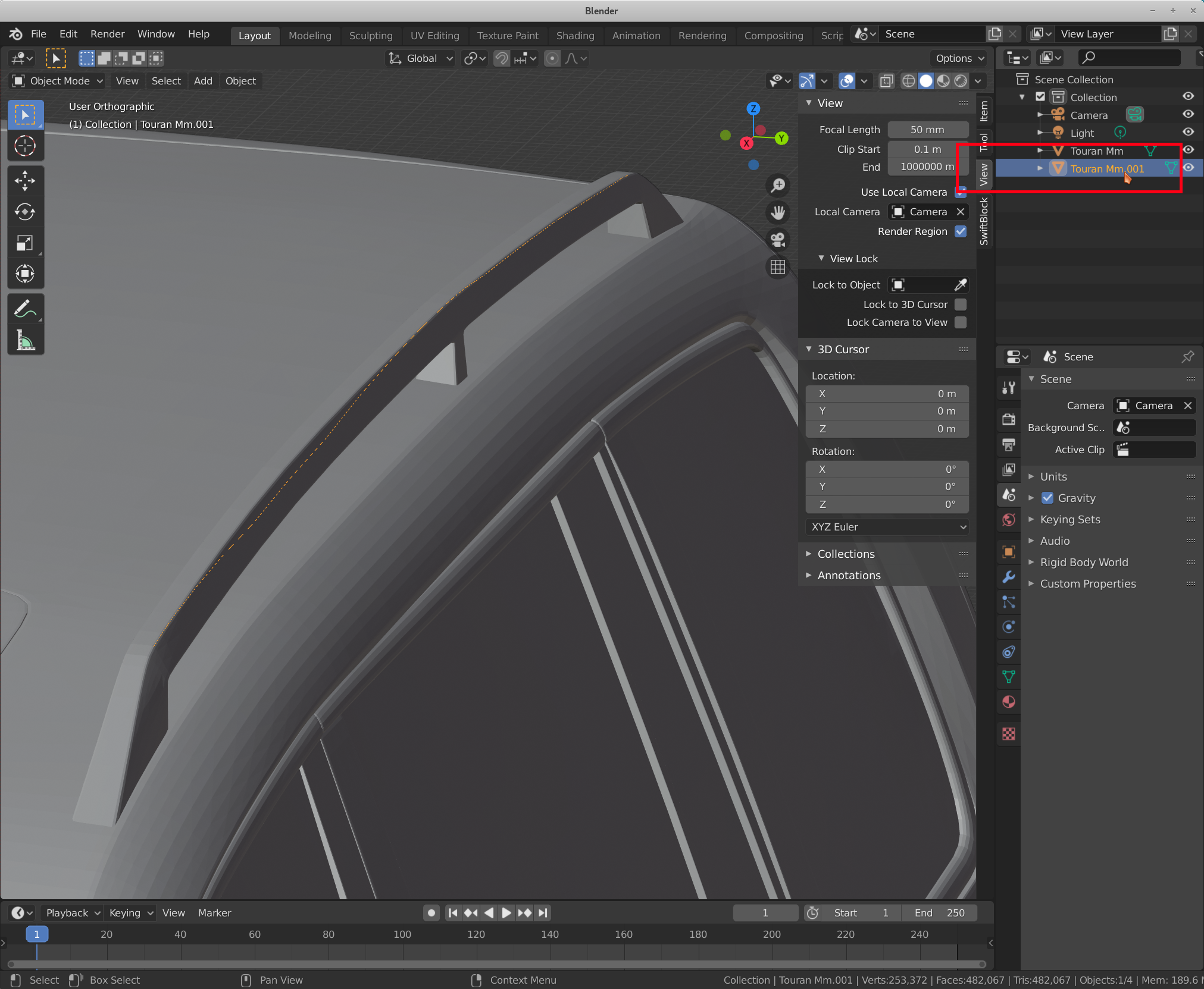
Here, it is described how to extract feature curves using the open source software Blender9 . The following steps are required:
Import the geometry into Blender
select in menu
select the STL file
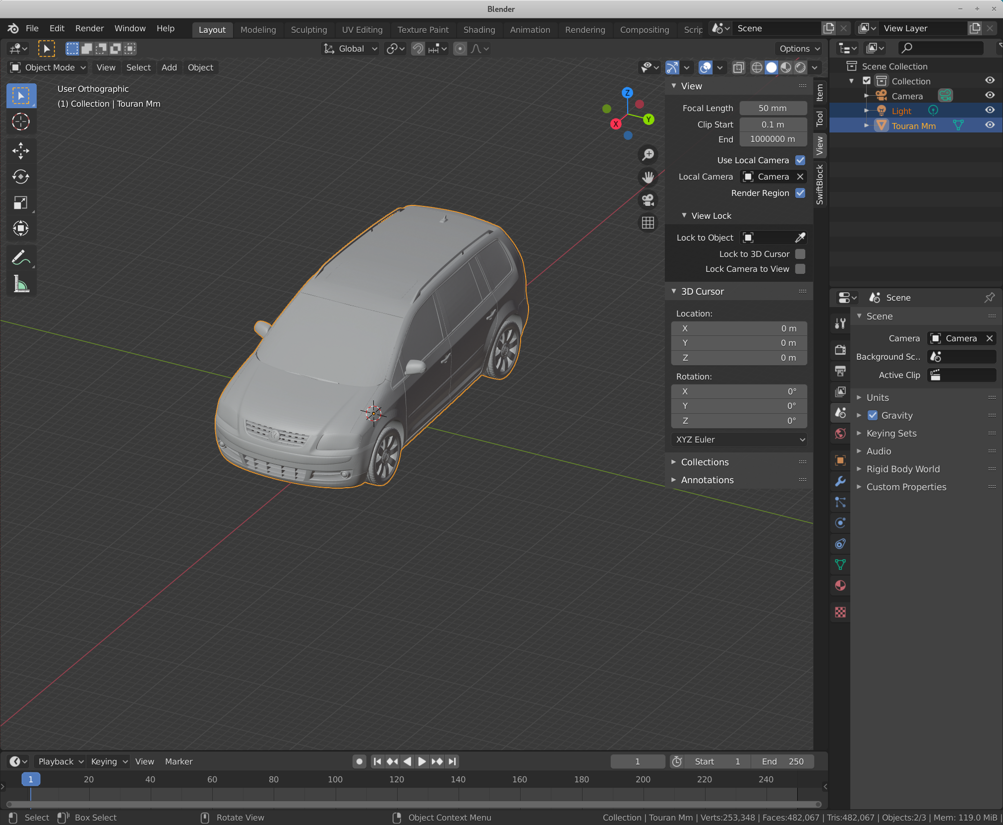
make sure, the object is selected (orange line around the selected object is displayed)
Objects can be selected by left click them with mouse.
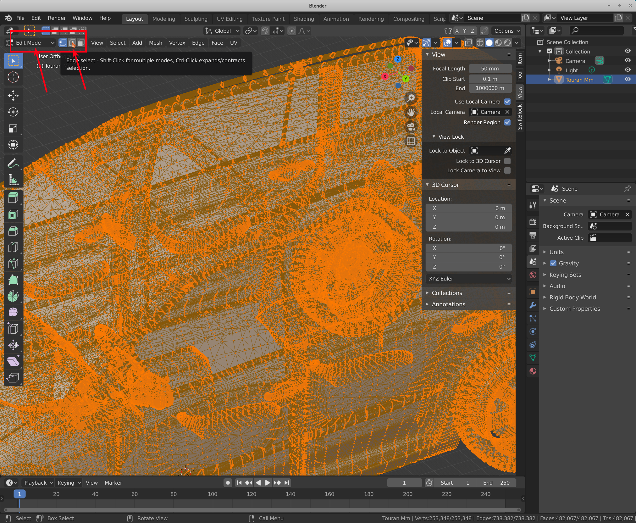
switch to ”Edit Mode”, either by pressing the ”Tab” key or by selecting the mode in the combo box in the upper left corner.
Next, switch to edge selection mode (second button right from the edit mode combo box)
In this example, we want to select a line (chain of edges) along the left roof rail.
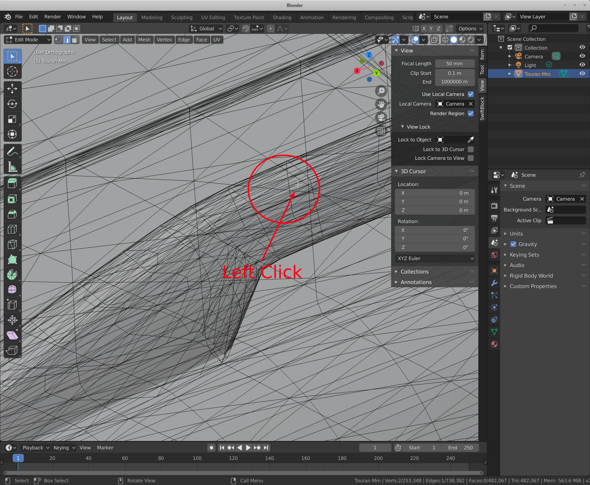
zoom into the location of the beginning of the line
select the first edge with a left click on it.
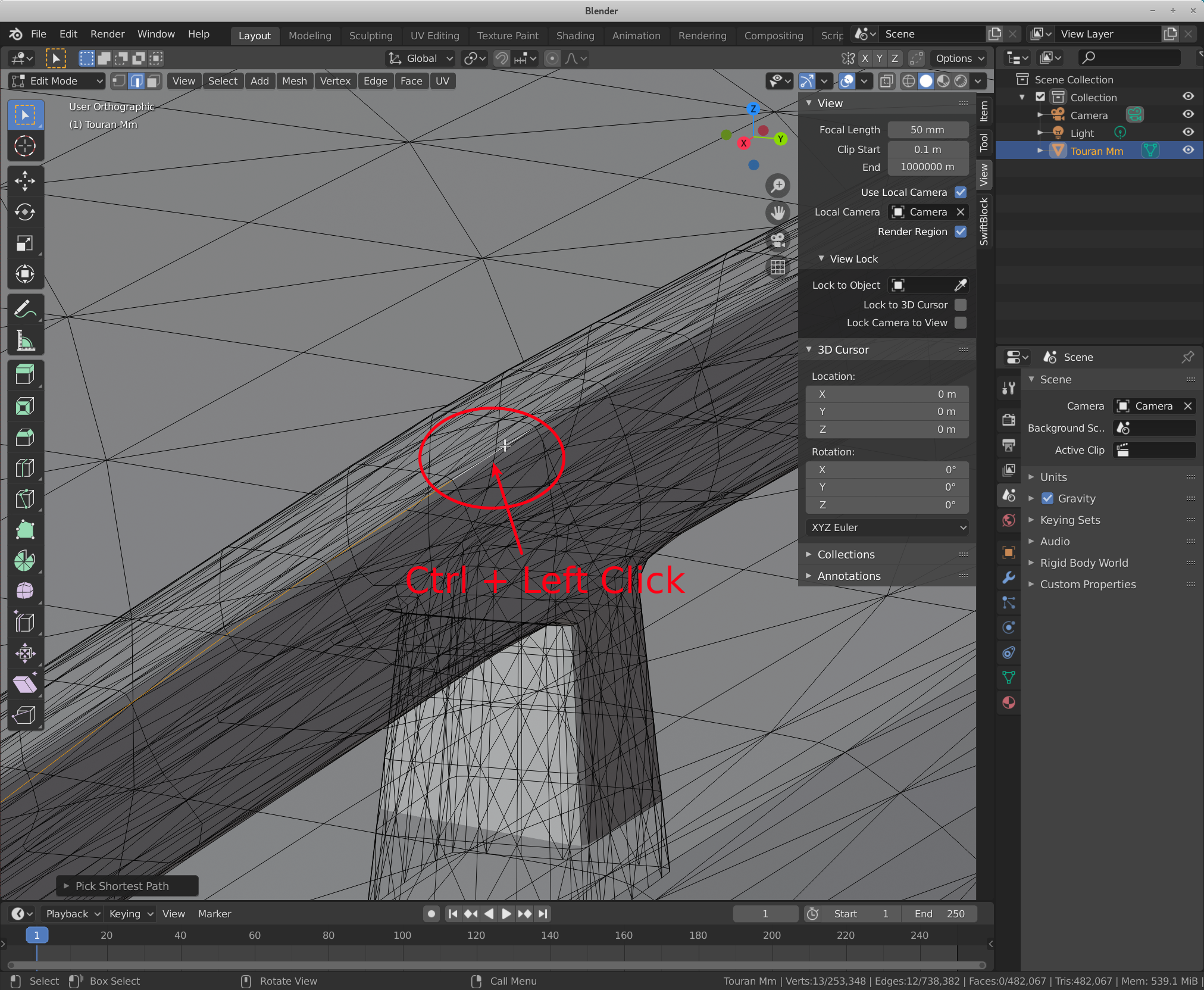
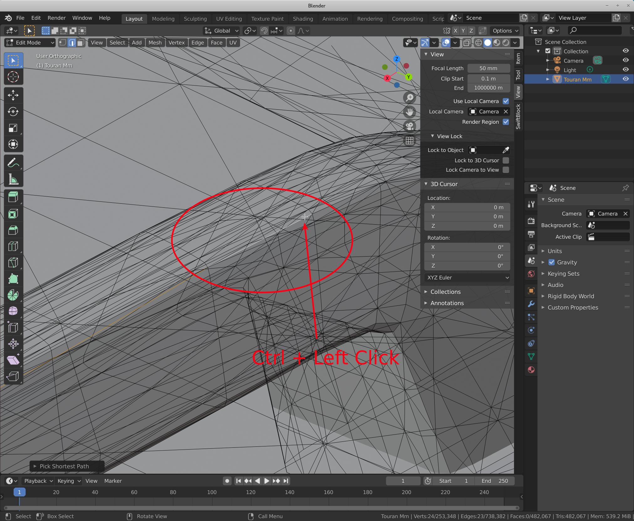
select another edge on the feature line: zoom to the next location and press Ctrl + Left click
The shortest path from the last selected edge and the current clicked edge will be added to the selection. To select edges as precise as possible, it might be required to click a number of intermediate locations. If a mistake is made, the last step can be undone by typing Ctrl+Z.
repeat the last step until the end of the feature line is reached.
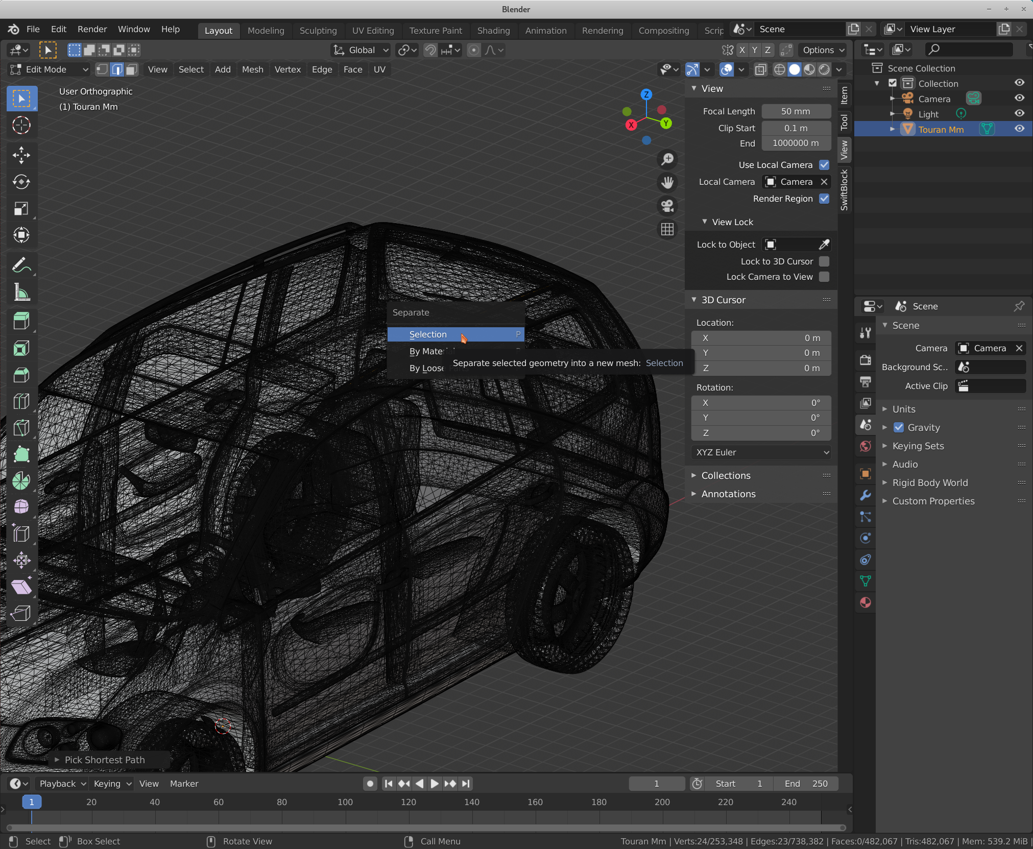
next create a new object from the selected edges by typing the key ”P”.
Then select ”Selection” to create the new part from the current selection.
Once the selection is split off, another chain of edges can be selected by repeating the steps from 5.
switch back to ”Object Mode”
either by pressing the Tab key or by selecting ”Object Mode” in the combo box in the upper left corner.
When multiple lines had been split into multiple new objects, these should be joined into a single one. To do so, select the objects in the object browser (upper right), then type ”Ctrl+J”.
Note: the mouse should be over the 3D viewport for Blender to accept the keyboard shortcut.
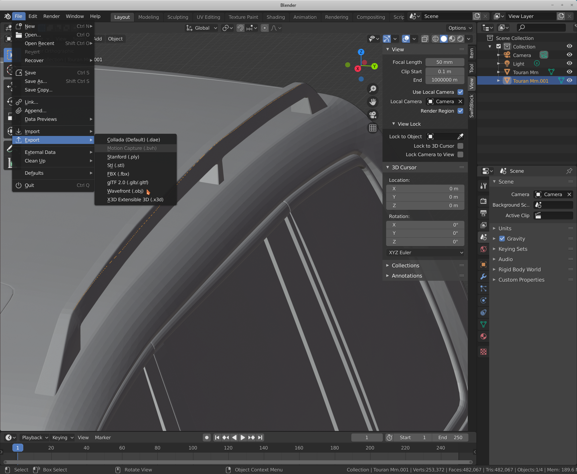
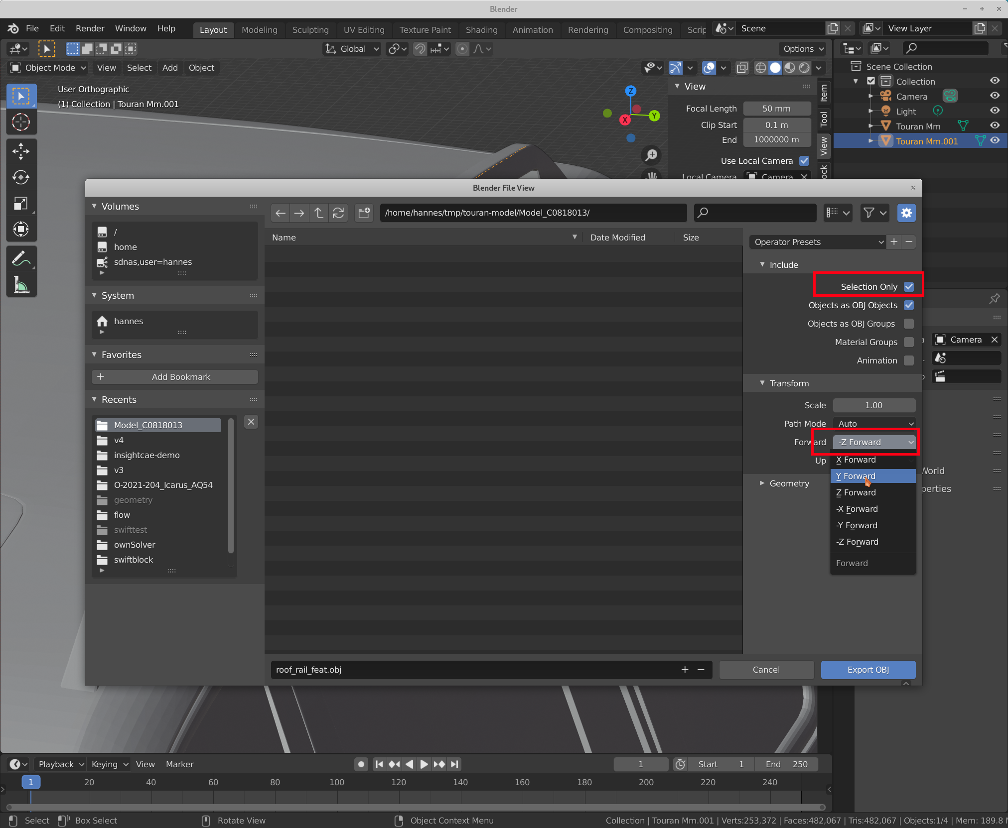
export the edges into an OBJ file.
Select the object in the object browser with a left click.
Then open the menu .
check the export settings. Make sure, the following is set:
”Selection only” is checked
(Otherwise also the surface will be included in the exported file)
In ”Transform”, ”Forward” is set to ”Y Forward”
(Otherwise the geometry will be wrongly oriented after export)
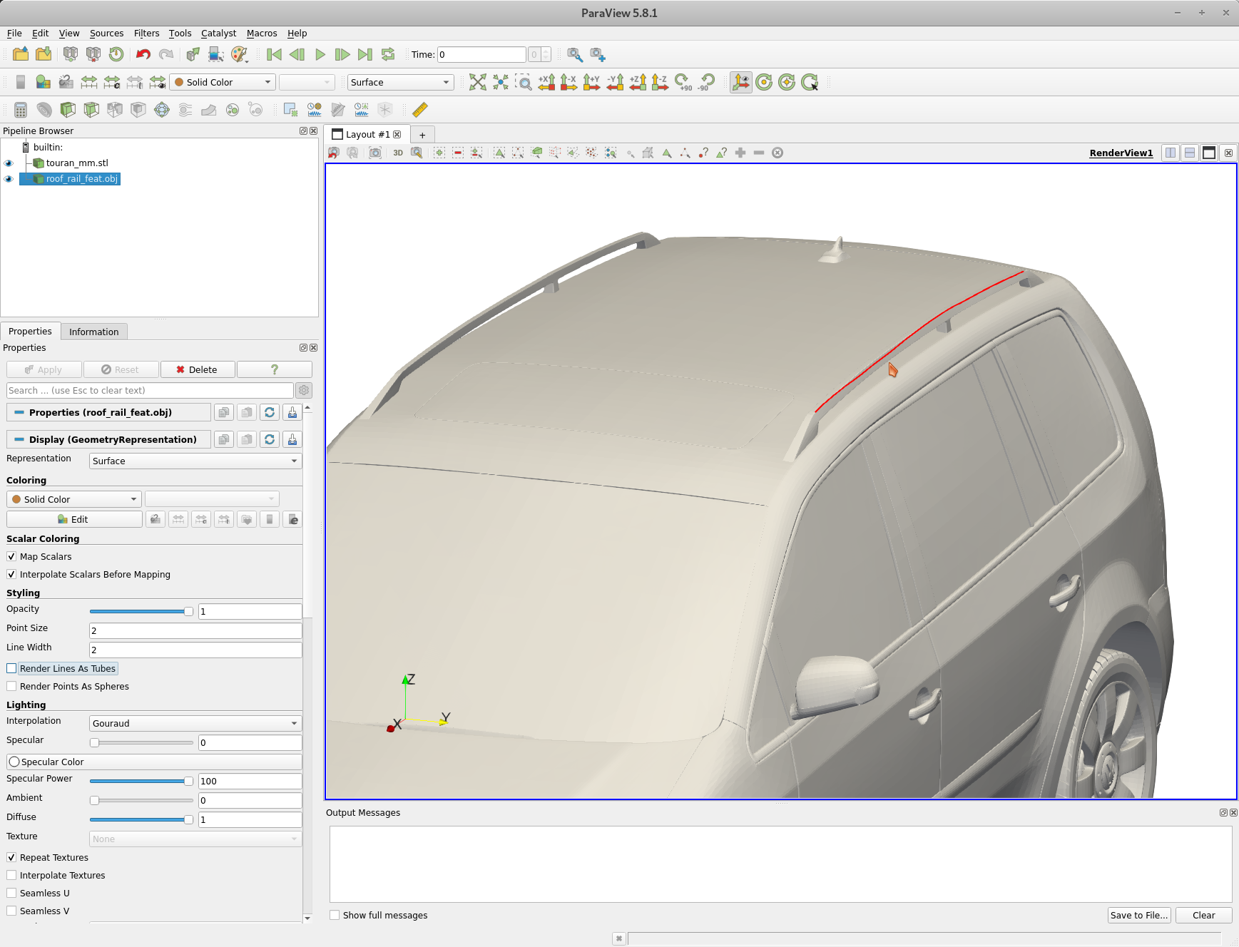
the resulting OBJ files can be loaded into Paraview and checked
Finally, the OBJ files can be converted into OpenFOAM’s eMesh format. There is a tool called ”surfaceFeatureConvert” in the OpenFOAM toolbox, which can perform this task. The file type is recognized from the extension. If not already done, the OpenFOAM environment needs to be loaded (here using the alias of1806):
InsightCAE bundles a number of extensions to OpenFOAM which are used in cases created by the toolkit.
8.1.1FieldDataProvider
The FieldDataProvider class provides a swiss-army-knife-like source for field data. It is used in a number of places, where field data is required as a parameter. Some examples are described in the next section.
The field data is described by a single line of text. The provided data can be steady or unsteady and homogeneous or inhomogeneous.
The different provider types together with their required value data are described in the following.
The keywords unsteady or steady select whether the input is time dependent. The steady keyword is the default and can be omitted. For unsteady input, the time instance data is a pair of a scalar time value and the value data. In the steady case, only the value data is required.
These provider types are known:
uniform The value data is single value.
Example:
1uniform(1 0 0)
nonuniform The value data is a list of values. The required number of entries is dependent on the context in which the FieldDataProvider is used. For a boundary condition for example, it needs to match the number of faces.
Example:
1nonuniform7(0 0 0 1 1 2 3)
linearProfile The value data is the name of a file which contains table of coordinate/value pairs, one per row. Between the lines is linearly interpolated.
This type requires additional input data:
the origin of the coordinate axis,
the direction of the coordinate axis.
Note: For vector and tensor values, the table file needs to contain one column per component in addition to the first column which contains the coordinate. The components are used as they are and are not transformed. For coordinates beyond the bounds of the table, the corresponding values at the bounds of the table are used (”clamp” behaviour).
This defines a linear profile starting at the global origin and the coordinate running along the y axis. The table file content could look like this (for a vector field):
110 0 020.91 0 03-0.91 0 04-10 0 0
radialProfile
circumferentialProfile The input for each instant is a file containing a table of components vs. angle. The coordinate system specification requires the base point, the axis direction and the direction of angle 0. The mapping is done this way: for each face, the angle is computed, the values for the angle are interpolated from the table and applied to the boundary. If the
value is a tensor, it is transformed according to the current angle.
In this example, die coordinate system has its origin at (000)T , the axis points along the global Z direction and the angle 0 is along the global X direction. The profile points are read from the file T_vs_phi.txt in the case directory.
fittedProfile
vtkField The data is read from a VTK file and interpolated to the CFD grid. The VTK grid needs to geometricall coincide with the target CFD mesh. There may be many fields in the VTK dataset and the one to be used has to be specified.
Example:
1vtkField"$FOAM_CASE/data.vtk" "U"
8.1.2extendedFixedValue
The extendedFixedValue boundary condition uses the FieldDataProvider class (see section 8.1.1) to apply the provided fields as a Dirichlet boundary condition in OpenFOAM cases.
The following settings need to be set in an OpenFOAM cases that uses this BC:
the library containing the BC needs to be added in the system/controlDict
1libs( "libextendedFixedValueBC.so" );
use the extendedFixedValue boundary condition type in some field file:
The source entry in the boundary section of the field file defines the actual FieldDataProvider input (see 8.1.1 for the syntax of the input statement).
The value statement needs to be present but will be replaced upon solver start with the value(s) evaluated from the FieldDataProvider machinery.
Part II Insight CAD
9InsightCAD
9.1Introduction
InsightCAD is a script-based tool for creating three-dimensional geometry models. All geometric operations are based on the OpenCASCADE geometry kernel. It uses the boundary representation approach (BREP) for treating the geometry. Thus it is possible to import and export the common exchange formats IGES and STEP.
Although the primary intention of InsightCAD is creation of fully parameterized CAD models for systematic numerical simulations, it can also be used for mechanical design purposes. It therefore provides the possibility to export projections and sections of the created models in DXF format for use in drawings. Additionally, there is support for a library of parametric standard parts.
9.2Basic Concept
The basic entity in InsightCAD is a ”model”. A model is described by a script and stored in an ASCII script file (extension ”.iscad”). Inside a model script, symbols are defined, which can represent the following data types:
Scalars
Vectors
Datum objects (axes, planes)
3D geometry objects (features)
Selections of vertices, edges, faces or solids of 3D geometry objects
There is no explicit type declaration: the data type of each symbol is deduced from the defining expression.
Beyond their geometry representation, geometry feature objects are containers for scalar, vector, datum and feature objects. These symbols can be accessed in the model script but are read-only.
In a model script, after the definition of the aforementioned symbols, an optional section with postprocessing actions can follow. These can be e.g. file export, drawing export or others.
General CAD Model Script Syntax The general model script layout begins with a mandatory symbol defining section, followed by an optional postprocessing section, started by ”@post”:
Comments are lines starting with ”#” or text regions enclosed by ”/*” and ”*/” (C-style).
9.3Submodels and Subassemblies
It is possible to load another model into the current one by the ”loadmodel” command (see section ”Features”). In this case, the loaded model represents a subassembly, i.e. a compound of features. Since not all defined geometry objects in the submodel may represent assembly components, marking of components is supported by the feature definition syntax and needs to be utilized properly in the definition script of the submodel. Also, when loading models (subassemblies), parameters can be
passed to the submodel. These can be scalars, vectors, datums or features.
9.4Symbol Definition
9.4.1Scalars
Example:
1D?= 123.5;2L= 2.*D;
The ”?=” operator assigns a default value. This needs to be used for symbols which are intended to be used as parameters in the ”loadmodel” feature command. Symbols defined by the equal sign operator (”=”) cannot be overridden during the loadmodel command.
There are scalars predefined in each model. They are included in table 6.
9.4.2Vectors
Example:
1v?= 5*EX + 3*EY + [0,0,1];2ev= v/mag(v);
The ”?=” operator assigns a default value. This needs to be used for symbols which are intended to be used as parameters in the ”loadmodel” feature command. Symbols defined by the equal sign operator (”=”) cannot be overridden during the loadmodel command.
reference point of datum (base point of axis or plane)
refdir(⟨datum⟩)
reference direction of datum (direction of axis or normal of plane)
Table 4:Vector operations and functions in ISCAD scripts
There are vectors predefined in each model. They are included in table 6.
9.4.3Datums
Some simple examples are given below.
1myaxis?= RefAxis(O, EX+EY); # diagonal axis2myplane= Plane(5*EX, EY); # offset plane3myplane2= XZ << 5*EX; # same offset plane4axis2= xsec_plpl(XY, myplane); # axis at intersection of XY-Planeandoffset plane
The ”?=” operator assigns a default value. This needs to be used for symbols which are intended to be used as parameters in the ”loadmodel” feature command. Symbols defined by the equal sign operator (”=”) cannot be overridden during the loadmodel command.
Geometry symbols can be defined by a ”=” or a ”:” operator. The difference comes from a possible use of the model as a subassembly later on. Since usually not all defined features in a model are assembly components but some are only intermediate modeling steps, there are these two syntaxes for defining a feature with a subtle difference: ”⟨identifier⟩ = ⟨expression⟩;” defines an intermediate feature while ”⟨identifier⟩: ⟨expression⟩;” does the same geometry operation but marks the result as being an assembly component. In the above example, only the feature ”pierced_cylinder” is marked as a component. Thus if the above example would be loaded as a subassembly, only the ”pierced_cylinder” will be shown
and included in e.g. mass calculations.
InsightCAD script
Description
⟨feature:a⟩ - ⟨feature:b⟩
Boolean subtract of feature b from feature a
⟨feature:a⟩|⟨feature:b⟩
Boolean unite of feature a and feature b
⟨feature:a⟩ & ⟨feature:b⟩
Boolean intersection of feature a and feature b
⟨feature⟩<<⟨vector:delta⟩
Copy of feature, translated by vector delta
⟨feature⟩ * ⟨scalar:s⟩
Copy of feature, scaled by s (relative to global origin O)
⟨feature⟩.⟨identifier:subfeatname⟩
Access of subfeature
Table 7:Vector operations and functions in ISCAD scripts
9.5Feature Commands
In this section, an incomplete subset of the avilable feature commands is described in detail. For a complete list, please refer to the online documentation in the iscad editor (press Ctrl+F).
Reads a sketch (i.e. a singly closed contour) from a file. The geometry in the sketch is expected to be drawn in the X-Y-Plane. It is placed on the given plane pl. Sketch file format is recognized from the file name extension. Supported are ”.dxf” and ”.fcstd” (FreeCAD). The name is interpreted as layer name in DXF and sketch name in FreeCAD files.
For FreeCAD sketches, a list of parameter values can optionally be supplied. Upon loading, the sketch will be regenerated through FreeCAD with these values.
Parses another InsightCAD model (submodel) and inserts a compound of all features into the current model, which were marked as components in the submodel (i.e. which were defined with the colon ”:” operator instead of the equal sign ”=” in the submodel).
The model filename has to be ”⟨modelname⟩.iscad”. It is searched for in the following directories:
the directories listed in the environment variable ”ISCAD_MODEL_PATH” (separated by ”:”)
the subdirectory ”iscad-library” in InsightCAEs shared file directory
in the current directory
Optionally, a list of symbols is inserted into the namespace of the submodel (additional optional parameters).
9.5.3Geometry Construction
Primitives There are commands for creation of several different geometrical primitives, e.g.
1D: Arc, Line, SplineCurve
2D: Quad, Tri (triangle), RegPoly (regular polygon), Circle, SplineSurface
3D: Sphere, Cylinder, Box, Bar, Cone, Pyramid, Torus
Extrusion(⟨feature:f⟩,⟨vector:L⟩[, centered ] )
Extrude the feature f with direction and length vector L. When the keyword ”centered” is given, the extrusion is centered around f.
Creates a revolution of the planar feature f. The rotation axis is specified by origin point 0 and the direction vector axis. Revolution angle is specified by phi. By giving the keyword ”centered”, the revolution is created symmetrically around the base feature.
Other Feature Commands There are more features available. A comprehensive list is obtained by pressing Ctrl+F in the iscad editor.
9.6Lower Dimensional Shape Selection
ISCAD supports rule based selection of lower dimensional features (i.e. edges or faces of a solid). The selection is generated by a selection command: a question mark, followed by the type of shape to query. The result is a selection object:
It is possible to supply additional arguments to the selection expression, like scalars, vectors or features.
An example: the following expression selects the circumferential face of the cylinder c (all faces, which are not plane) and stores the selection in ”shell_faces”:
1c= Cylinder(O, 5*EZ);2shell_face= c ? faces(’!isPlane’);3min_end_face= c ? faces(’isPlane␣&&␣minimal(CoG.z)’);
The selection command string contains rules for the selection. Finally, the command string is evaluated as a boolean expression comprising comparison operators, boolean operators and query functions. Within these boolean expressions, quantity functions can be used. The available set of query functions and quantity functions depends on the type of shape which shall be queried.
Boolean expressions available for all kinds of lower dimensional shapes are listed in table 8.
Quantity functions available for all kinds of lower dimensional shapes are listed in table 9.
Command
Description
==, <, >, >=, <=
value comparison
!
not
&&
and
||
or
⟨value 1⟩ ˜ ⟨value 2⟩{⟨tolerance⟩}
approximate equality
in(⟨selection set⟩)
true if shape is in other selection
maximal(⟨quantity⟩)
true for the shape with maximum quantity
minimal(⟨quantity⟩)
true for the shape with minimum quantity
Table 8:General boolean functions and operators available for all kinds of lower dimensional shape
Command
Description
angleMag(⟨vec 1⟩, ⟨vec 2⟩)
angle between vec 1 and vec 2
angle(⟨vec 1⟩, ⟨vec 2⟩)
angle between vec 1 and vec 2
%d⟨index⟩
parameter ⟨index⟩ as scalar
%m⟨index⟩
parameter ⟨index⟩ as vector
%⟨index⟩
parameter ⟨index⟩ as selection set
Table 9:General quantity functions available for all kinds of lower dimensional shape
9.6.1Vertices
There are no special boolean functions or operators for vertices.
The available quantity functions for vertices are listed in table 10.
Command
Description
loc
location of the vertex
Table 10:Quantity functions available for vertex selections
9.6.2Edges
Boolean functions for edges are listed in table 11.
The available quantity functions for edges are listed in table 12.
Command
Description
isLine
true, if edge is straight
isCircle
true, if edge is circular
isEllipse
true, if edge is elliptical
isHyperbola
true, if edge is on a hyperbola
isParabola
true, if edge is on a parabola
isBezierCurve
true, if edge is a bezier curve
isBSplineCurve
true, if edge is a BSpline curve
isOtherCurve
true, if edge is none of the above
isFaceBoundary
true, if edge is boundary of some face
boundaryOfFace(⟨set⟩)
true, if edge is boundary of one of the faces in set
isPartOfSolid(⟨set⟩)
true, if edge is part of one of the solids in set
isCoincident(⟨set⟩)
true, if edge is coincident with one of the edges in set
isIdentical(⟨set⟩)
true, if edge is identical with one of the edges in set
The DXF postprocessing action creates a DXF file for further use in drawings. Several views are derived from the feature f. A ⟨view_definition⟩ takes the following form:
1<identifier:viewname>(2<vector:p_0>,<vector:n>, up <vector:e_up>3[,section]4[,poly]5[,skiphl]6[,add [l] [r] [t] [b] [k] ]7)
It defines a view on the point vector 0 with normal direction vector of the view plane. The upward direction (Y-direction) is aligned with vector up.
The keyword ”section” toggles whether only the outline is projected or if the view plane creates a section through the geometry.
If keyword ”poly” is given, the DXF geometry will be discretized. This is more robust but creates much larger DXF files.
Keyword ”skiphl” toggles whether hidden lines are output.
The keyword ”add” followed by the key letters l, r, t, b and/or k enables creation of additional projections from the left, right, top, bottom and/or back, respectively.
An example is given below:
1c:Cylinder(O, 100*EX, 20);23@post45DXF("c.dxf")<< c6top( O, EX, up EY )7front( O, EZ, up EY )8;
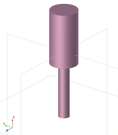
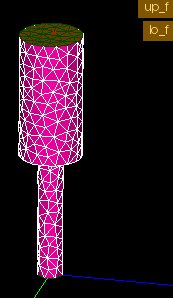
Generates a (triangular or tetrahedral) mesh for an FEA analysis of the feature f. Gmsh is used as a meshing backend. The mesh format is determined by the outputfile extension (.med = MED format). The label of the mesh is set to l.
The syntax of the ⟨mesh_parameters⟩ are as follows:
The general mesh size is set by Lmax and Lmin. The optional keyword ”linear” switch from quadratic to linear elements. Named groups of vertices, edges and faces can be created using the keywords ”vertexGroups”, ”edgeGroups” and ”faceGroups” repectively. Each group definition takes the form ”groupname” = ”selection set” (see section ”Lower dimensional shape selection” for definition of selection sets). Optionally, a mesh size can be assigned to each defined group by appending an @ sign
followed by a scalar value.
An example is given below:
1c:2Cylinder(O,100*EX, 20)3|4Cylinder(100*EX,ax 100*EX, 50)5;67@post89gmsh("c.med")<< c as cyl10L= (10 0.1)11linear12vertexGroups()13edgeGroups()14faceGroups(15lo_f= c?faces(’isPlane&&minimal(CoG.x)’)16up_f= c?faces(’isPlane&&maximal(CoG.x)’)17)18;
Result: ISCAD model (left) and resulting mesh (right):
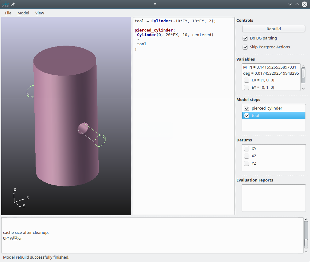
9.8Graphical Editor ISCAD
ISCAD is a graphical editor for InsightCAD scripts. It consists of a text editor for editing the script contents and a 3D view and some other elements for inspecting the resulting model. A screenshot is shown in the figure below.
The model script is entered into the text editor widget right of the 3D display. Once a script shall be evaluated, it can be parsed by clicking in the button ”Rebuild” or pressing Ctrl+Return.
After parsing the model, the following results are displayed:
A list of all created feature symbols in the ”Model Steps” list box. If the check box is checked, the 3D geometry is displayed in the 3D view.
The values of all scalars and vectors in the ”Variables” list box.
For each vector variable, a check box is displayed. If it is checked, the vector is interpreted as a point location and the point is shown in the 3D display window.
All defined datums are listed in the ”Datums” list box. Again, the check box controls, whether the datum is displayed in the 3D view.
9.8.13D Graphics Display
View Manipulation
Dragging: Shift + mouse move
Scaling: Ctrl + horizontal mouse move
Rotating: Alt + mouse move
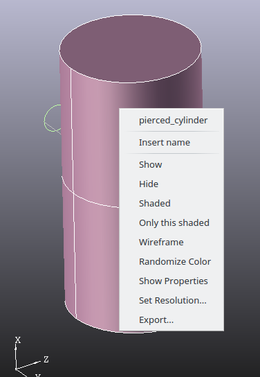
Model Navigation When hoovering the mouse pointer over a displayed feature in the 3D geometry window, it is highlighted. The highlighted feature is the one, which would be selected during subsequent mouse clicks.
When the left mouse button is pressed, the highlighted feature is selected and all its contained reference points are displayed.
When the right mouse button is pressed, a context menu for the selected feature is displayed.
The context menu provides these functions:
The first entry is the feature name. When it is selected, the definition in the script editor is highlighted and the cursor jumps to it.
”Insert name”: inserts the name of the feature symbol at the cursor location
”Export...”: Export the feature geometry to a file (BREP, STP, IGES, STL)
9.8.2Text Editor
When script code is entered into the text editor window, it is parsed in the background. Once this has been done successfully, some extensions of the context menu is available:
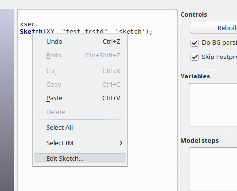
Context menu on ”Sketch” command:
When selecting the ”Edit Sketch...” entry, FreeCAD is launched and the sketch editor opened. If the FreeCAD-file or sketch inside it is not yet existing, they are created.
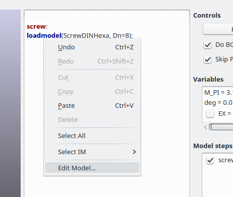
Context menu on ”loadmodel” command:
When selecting the ”Edit Model...” entry, another instance of iscad is launched with the specified model script loaded.
Part III API
InsightCAE is a toolbox for the creation of custom workflows. It is therefore very natural to use its API in own extensions.
There are different developer perspectives:
Creating extensions (own workflow modules).
To write own workflow modules, just a plain binary installation of InsightCAE is required. It brings header files for its libraries and a CMake configuration which enables the developer to build his own extensions. It is recommended to create a custom library containing the additions (plug-in). See section 10 for a guide.
Modifying and extending the InsightCAE base project itself.
Since InsightCAE is free and open software, it is perfectly possible to take it and apply extensions or corrections or any other modification or improvement. Please note that silentdynamics GmbH develops InsightCAE primarily with its own applications in mind so there are almost certainly features missing in the API which third party users might need. If you implement something which might be of public interest, please think about sharing it with us and the rest of the community. We are
very open to integrate foreign contributions into the project.
Now, modifying the InsightCAE project requires to build the project from its sources. Please see section 11 for a guide to set up a self-built working copy of the sources.
10Plug-In Development
11InsightCAE Development
11.1Dependencies
The InsightCAE toolkit requires a number of dependencies. Not all versions have been tested, of course. The following list contains the major dependencies along with the versions, which are currently utilized in binary packages:
The InsightCAE sources are prepared to be built in a Posix environment. The developers use Ubuntu Linux in the latest LTS version. The Windows version is cross-compiled using the MXE cross compiling suite.
11.2.1Building in Linux
Some prerequisites:
GCC 10 should be used. Newer version were found to have buggy optimizers.
For Ubuntu, there is a package containing all the important dependencies. Install it by
1$sudo apt install insightcae-dependencies
CMake Configuration and Building An out-of-source build is recommended. If the aforementioned dependencies package is used, the following variables need to be added to the CMake configuration:
INSIGHT_SUPERBUILD=/opt/insightcae
Once configured, the project is built either by
1$make
or
1$ninja
depending on the chosen generator.
Execution Once built, the InsightCAE programs can be executed directly from the build folder, provided that the environment is set.
To setup the environment, add the appropriate script to the beginning of the /.bashrc file:
Cross-Compiler First, an installation of MXE is required. There is Ubuntu installation package in the InsightCAE development repository (see section 3). It contains all the required dependencies plus some additional packages (i.e. dxflib and python 3.6) and a number of patches. It can be installed
using:
1$sudo apt install mxe
On other Linux distributions, MXE probably needs to be built from its sources. The following command should do the build of all required packages:
With these variables manually added, it should be possible to build the project with QtCreator.
Executing the Built Binaries in a Windows Machine Install a SAMBA server and export the following paths as shares:
the build directory (e.g. build-insight-Desktop_MXE32_shared-Release) as share ”insightwin”
Make sure to include the option acl allow execute always = True for the share. Otherwise there will be an error 0xc0000022 when it is attempted to execute an EXE file from the share.
Prepare a windows machine with the following steps:
install python3.6.8rc1.exe (32bit version is required!)
Make sure to enable the option ”add Python executable to PATH”!
map the share ”insightwin” ⇒ drive I:
Set the following environment variables:
INSIGHT_GLOBALSHAREDDIRS=i:∖share∖insight
append to PATH:
i:∖bin
i:∖lib
Once this is done, it should be possible to execute the EXE files directly from the network drive I:∖bin
To run flow simulations or finite element analyses, the Windows installation needs a linux environment since the backend tools are mostly only available for Linux. Therefore, a WSL container is required with an InsightCAE linux version inside. For development purposes, it is beneficial to have the InsightCAE linux build from the same source available inside the WSL container as was used to create the Windows version. The following steps can be made to achieve this goal:
Export the build folder (when QtCreator is used, it may be named like ”build-insight-Desktop_superbuild-Debug”) of the Linux build as an additional share by the Samba server (e.g. named ”insightlin”).
Create an Ubuntu WSL container, e.g. execute in a Power Shell:
1>wsl.exe --install --distribution=Ubuntu-22.04
Launch a shell in the newly created container:
1>wsl.exe
and install the insightcae-dependencies package (compare section 3.1).
The following commands at the WSL containers bash prompt are required:
Then mount the share and add the environment setup script to the users’ bashrc file:
1$sudo mkdir -p /opt/build-insightcae2$echo’\\<server>\insightlin␣/opt/build-insightcae␣drvfs␣defaults␣0␣0’ | sudo tee /etc/fstab3$sudo mount -a4$sed-i ’1i␣source␣/opt/build-insightcae/bin/insight_setenv.sh’ ~/.bashrc5$sed-i ’1i␣source␣/opt/insightcae/bin/insight_setthirdpartyenv.sh’ ~/.bashrc
Note: File I/O from within the WSL container is slowed down considerably by the Windows Defender Services. To improve performance, consider to disable this service and/or add exceptions where possible.
11.3Structure of the InsightCAE Project
The core of InsightCAE consists of a number of libraries. There is a core library (libtoolkit) which contains the basic functions. Other, optional features are found in a number of other libraries which differ in their build dependencies.
Overview over the component libraries:
toolkit (depends on VTK, Boost, Armadillo, GSL)
i.e. depends only on the basic dependencies (including VTK)
insightcad (depends on toolkit, OpenCASCADE, DXFlib)
i.e. depends on the basic features plus CAD kernel
Provides all the CAD functions but excluding CAD-related GUI classes.
tookit_remote (depends on toolkit, Wt)
Contains classes for remote execution client that require Wt
tookit_cad (depends on toolkit, insightcad)
Contains extensions to basic classes that require CAD (e.g. visualization of block mesh templates) but not GUI-related classes.
toolkit_gui (depends on toolkit, toolkit_cad, insightcad, toolkit_remote, Qt)
Extends all the above with Qt-GUI support.
11.4Creating and Distributing Snapshots of a Build
11.4.1Linux Build
Creation Move into the build directory and execute CPack, e.g.:
(Replace ¡UNPACK PATH¿ with the path, in which the tar xzf command was executed. Also the version number in the archive will be different)
A new shell needs to be opened to apply the changes.
11.4.2Windows Build using MXE
Creation There is a script for creating the MSI installer which also copied the required dependencies from the MXE installation. It is intended to be executed from the build directory. For example:
(The correct version number should be inserted after ”-v”)
This will yield an installation package ”insightcae.msi”.
Installation The resulting MSI package has to be copied to the target and installed using the Windows tools (double click in the explorer window on the file).
 in the menu).
 or by checking the appropriate option in the ”Save Parameters” dialog. Once, a parameter file was saved as packed or unpacked, the selection state is saved and used for all subsequent save operations.
 in the menu. This analysis form switches automatically to the ”Run” tab (see figure
  in the menu.
 . Then a new dialog appears, in which the list of available analyses is displayed (figure
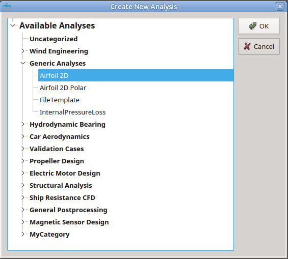

 and select the ISR file in the file selection dialog. The result elements are then shown in the tree view on the left side of the window (
 and enter a file path to the desired output PDF file.
Optionally, some result set elements can be omitted from the PDF rendering by applying filters, see
and enter a file path to the desired output PDF file.
Optionally, some result set elements can be omitted from the PDF rendering by applying filters, see 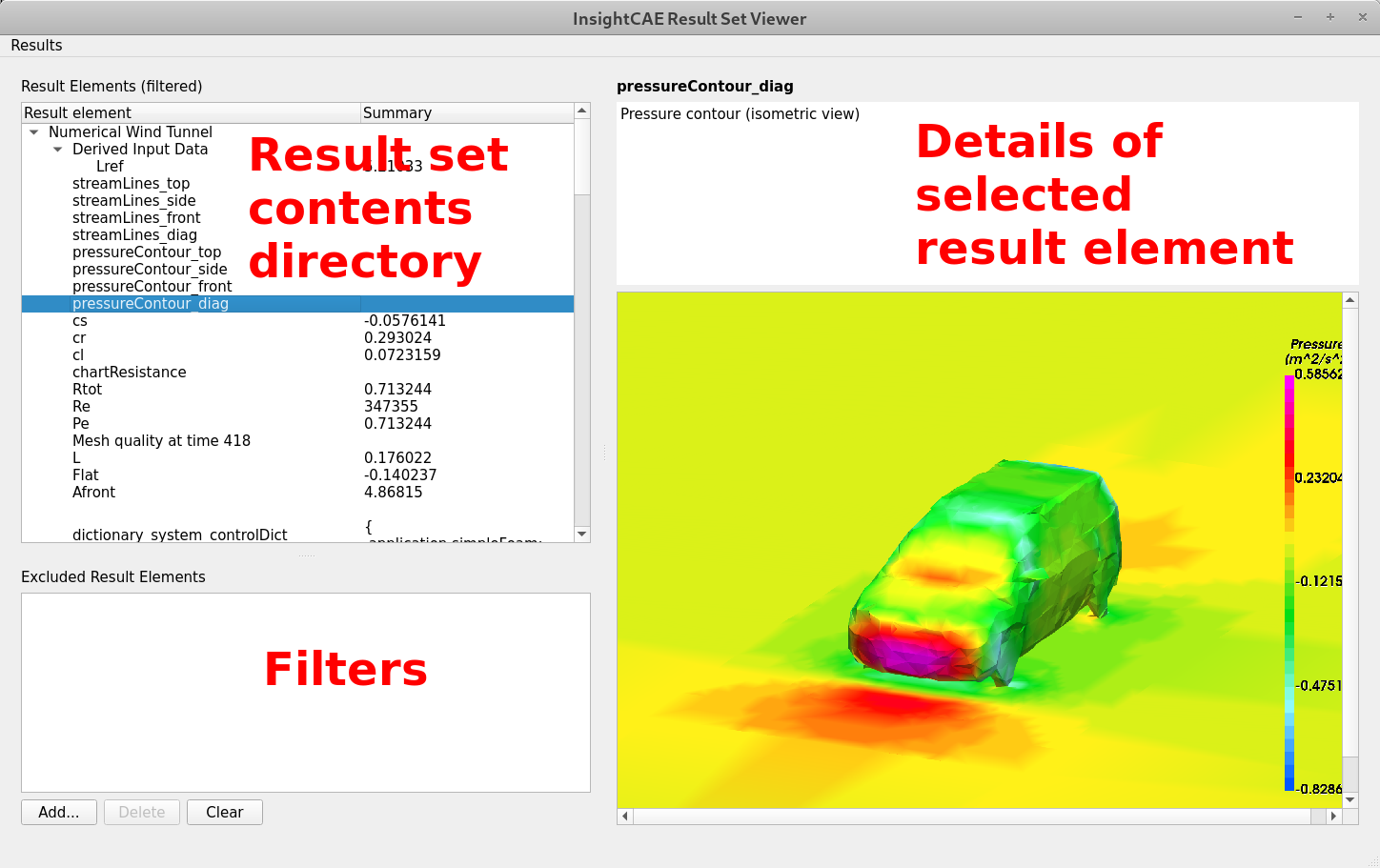
 .
. .
.
 . Make sure that the OpenFOAM case source is selected in the pipeline browser when the filter is added. When all the boundaries of interest are selected, click on ”Apply”.
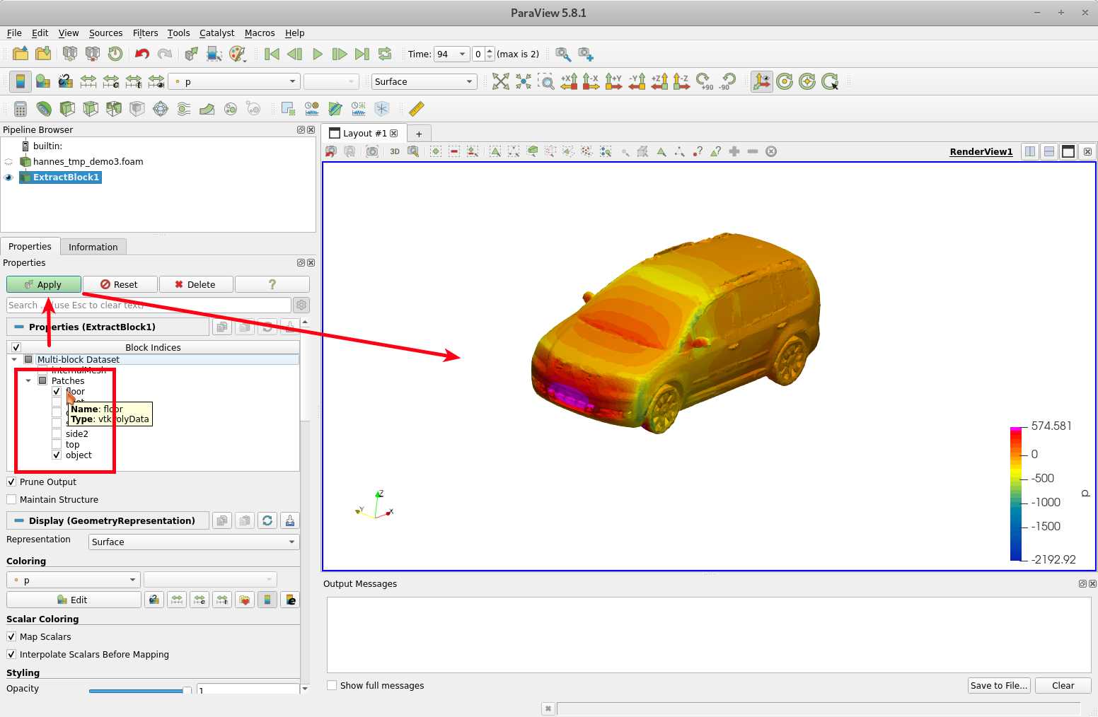


 .
.


 = (0
= (0


 of the view plane. The upward direction (Y-direction) is aligned with vector